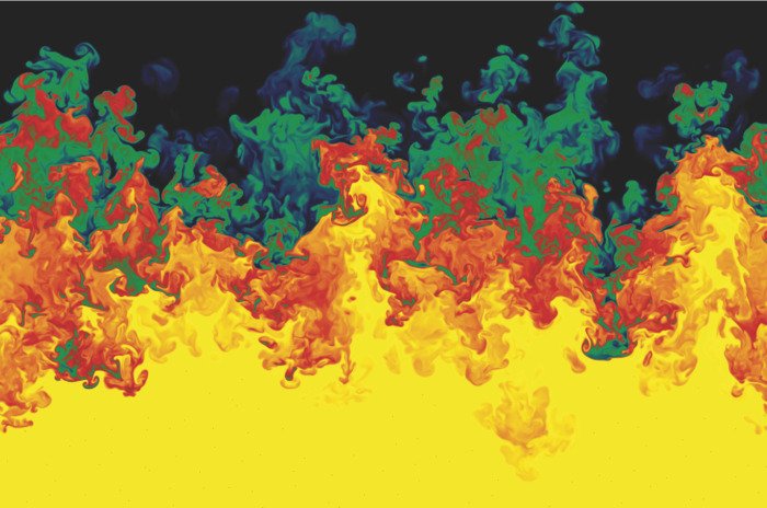
Though they may appear random at first glance, turbulent flows do possess structure. The video above shows a numerical simulation of a mixing layer, a flow in which two adjacent regions of fluid move with different velocities. The upper third of the frame shows a top view, and the bottom frame shows a side view, in which the upper fluid layer moves faster than the lower one. The difference in velocities creates shear which quickly drives the mixing layer into turbulence. But watch the chaos carefully, and your eye will pick out vortices rolling clockwise in the largest scales of the mixing layer. These features are known as coherent structures, and they are key to current efforts to understand and model turbulent flows. (Video credit: A. McMullan)
Tag: numerical simulation

Stingray Wakes
This numerical simulation shows a swimming stingray and the vorticity generated by its motion. Stingrays are undulatory swimmers, meaning that the wavelength of their motion is much shorter than their body length. Manta rays, in contrast, move their fins through a wavelength longer than their body length, making them oscillatory swimmers. Observe the difference in this video. To swim faster, stingrays increase the frequency of their undulation, not the amplitude. This is quite common among swimmers because increasing the amplitude also increases projected frontal area, which causes additional drag. Increasing the frequency of motion does not affect the projected area, making it the more efficient locomotive choice. (Video credit: G. Weymouth; additional research credit: E. Blevins; submitted by L. Buss)
Also, FYFD now has a Google+ page for those who prefer to follow along and share that way. – Nicole

Instability: Dense Over Light
Here on Earth, placing a dense layer of fluid atop a less dense layer is unstable. Specifically, the situation causes the interface between the two fluids to break down in what is known as the Rayleigh-Taylor instability.The video above shows a 2D numerical simulation of this breakdown, with the darker, denser fluid on top. The waviness of the initial interface provides a perturbation–a small disturbance–which grows in time. The two fluids spiral into one another in a fractal-like mushroom pattern. The continued motion of the dense fluid downward and the lighter fluid upward mixes the entire volume toward a uniform equilibrium. For those interested in the numerical methods used, check out the original video page. (Video credit: Thunabrain)

Turbulence and Magnetic Field Lines
During a solar flare, magnetic field lines on the sun are often visible due to the flow of plasma–charged particles–along the lines. According to theory, these magnetic lines should remain intact, but they are sometimes observed breaking and reconnecting with other lines. An interdisciplinary team of researchers suggests that turbulence may be the missing link. In their magnetohydrodynamic simulation, they found that the presence of chaotic turbulent motions made the magnetic line motion entirely unpredictable, whereas laminar flows behaved according to conventional flux-freezing theory. (Photo credit: NASA SDO; Research credit: G. Eyink et al.; via SpaceRef; submitted by jshoer)

Mixing the Southern Ocean
Motion in the ocean is driven by many factors, including temperature, salinity, geography, and atmospheric interactions. While global currents dictate much of the large-scale motion, it’s sometimes the smaller scales that impact the climate. This visualization shows numerically simulated data from the Southern Ocean over the course of a year. The eddies that swirl off from the main currents are responsible for much of the mixing that occurs between areas of different temperature, which ultimately impacts large-scale temperature distributions, in this case affecting the flux of heat toward Antarctica. (Video credit: I. Rosso, A. Klocker, A. Hogg, S. Ramsden; submitted by S. Ramsden)

Mixing Physics
When a dense fluid sits above a lighter fluid in a gravitational field, the interface between the two fluids is unstable. It breaks down via a Rayleigh-Taylor instability, with mushroom-like protrusions of the lighter fluid into the heavier one. The image above comes from a numerical simulation of this effect well after the initial instability; the darker colors represent denser fluids and lighter colors are less dense fluids. The flow here has progressed to turbulence, and the authors of the simulation are exploring the statistical nature of this flow breakdown relative to the classical case of isotropic, homogeneous turbulence. (Photo credit: W. Cabot and Y. Zhou)

Airborne Aerosols
This numerical simulation from NASA Goddard shows the motion of particulates in Earth’s atmosphere between August 2006 and April 2007. These aerosols come from various sources including smoke, soot, dust, and sea salt. As these fine particles move through atmosphere, they can have significant effects on weather as well as climate. For example, the particles serve as nucleation sites for the condensation and formation of rain drops. (Video credit: NASA Goddard SFC)

Stirring Faces
This video features simulation of the laminar flow around a plate plunging sinusoidally in a quiescent flow. As the plate moves up and down, it mixes the fluid around it. This is visualized in several ways, beginning with the vorticity. Clockwise and anti-clockwise vortices are shed by the edges of the plate as it moves. The flow is also visualized using particle trajectories, which are classified by their tendency to accumulate (attract) or lose (repel) particles. These trajectories are particularly intriguing to watch develop as they appear to show ornate faces and designs. (Video credit: S. L. Brunton and C. W. Rowley)

Supersonic Bubble Shock Waves
Supercomputing has been an enormous boon to fluid dynamics over the past few decades. Many problems, like the interaction between a supersonic shock wave and a bubble, are too complicated for analytical solutions and difficult to measure experimentally. Numerical simulation of the problem, combined with visualization of key variables, adds invaluable understanding. Here a shock wave strikes a helium bubble at Mach 3, and the subsequent interactions in terms of density and vorticity are shown. This situation is relevant to a number of applications, such as supersonic combustion and shockwave lithotripsy–a medical technique in which kidney stones are broken up inside the body using shock waves. After impact, an air jet forms and penetrates the center of the structure while the outer regions mix and form a persistent vortex ring. (Video credit: B. Hejazialhosseini et al.; via Physics Buzz)

Unsteady Rocket Nozzle
This numerical simulation gives a glimpse of flow inside an unsteady rocket nozzle. The nozzle is over-expanded, meaning that the exhaust’s pressure is lower than that of the ambient atmosphere. A slightly over-expanded nozzle causes little more than a decrease in efficiency, but if the nozzle is grossly over-expanded, the boundary layer along the nozzle wall can separate and induce major instabilities, as seen here. In the first segment of the video, turbulent structures along the nozzle wall boundary layer are shown; note how the boundary layer becomes very thick and turbulent after the primary shock wave (shown in gray). This is due to the flow separating near the wall. The second half of the video shows the unsteadiness this can create. The primary shock wave splits into two near the wall, creating a lambda shock wave, named for the shape of the lower case Greek letter. This shock structure is indicative of strong interaction between the boundary layer and shock wave. (Video credit: B. Olson and S. Lele)