Tag: numerical simulation

  • Plesiosaur Swimming

    Plesiosaur Swimming

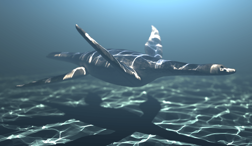
    Plesiosaurs are marine reptiles that thrived during the Jurassic period and went extinct some 66 million years ago. Since the first discoveries of plesiosaur fossils centuries ago, scientists have debated how the four-limbed creature would have swam. One approach to answering this question is to examine the efficiency of different strokes. Researchers have done this computationally by building a digital plesiosaur with biologically realistic joint motions. They then couple the model plesiosaur’s body motions with the movement of fluid around the body. With this computational model, they then simulate many different methods for moving the plesiosaur’s limbs and search for the most efficient one.

    What they found is that the plesiosaur’s propulsion is dominated by its forelimbs, which likely moved with a flight stroke similar to that of a penguin or sea turtle. Despite their size, the hindlimbs were able to produce very little thrust, suggesting that they were primarily used for stability and maneuverability. (Image credits: S. Liu et al., GIF source)

  • Amphibious Adaptation

    Amphibious Adaptation

    Every year newts move to the water in the springtime to mate before returning to land for the rest of the year. This annual aquatic relocation is accompanied by changes in the newt’s body. Flaps of skin grow from their upper jaw to their lower jaw, partially closing their mouths at the corners. This can be seen in the left column of the animation compared to the center and right.

    Numerical simulation shows that this mouth change has a significant impact on the newt’s ability to hunt underwater. Newts are suction feeders, who open their jaws and expand their mouth cavity to suck in water and their prey. By closing off the corners of their mouths during their aquatic phase, the newts generate more suction, reaching peak flow velocities 10% to 50% higher than in their terrestrial form and enabling them to pull prey from 15% further away. When they leave the water, the newts lose the extra flaps so that their mouths can open wider for catching prey on land. (Image credit: S. Van Wassenbergh and E. Heiss, source)

  • Turbulence in the Solar Wind

    Turbulence in the Solar Wind

    One of the key features of turbulent flows is that they contain many different length scales. Look at the plume from an erupting volcano, and you’ll see eddies that are hundreds of meters across as well as tiny ones on the order of millimeters. This enormous difference in scale is one of the major challenges in simulating turbulent flows. Since energy enters at the large scale and is passed to smaller and smaller scales before being dissipated at the tiniest scales of the flow, properly simulating a turbulent flow requires resolving all of these length scales. This is especially challenging for applications like the solar wind – the  stream of charged particles that flows from the sun and gets diverted around the Earth by our magnetic field. The image above shows some of the turbulence in our solar wind. The structures seen in the flow range from the size of the Earth all the way to the scale of electrons! (Image credit: B. Loring, Berkeley Lab)

  • Ocean Mixing

    Ocean Mixing

    Movement in Earth’s oceans is driven by a complicated interplay of many factors like temperature, salinity, and Earth’s rotation. Above are results from a numerical simulation of the top 100 meters of ocean contained within a 1 km x 1 km box.  The colors indicate surface temperature. Two major processes create the motion we see. The first is convection, in which water at the surface releases heat to the atmosphere and cools, causing it to then sink due to its greater density. Warmer water rises to replace it. This process happens quickly and dominates the early part of the simulation where we see the puffy convection cells shown on the left animation.

    A slower process is in effect as well. Because of variations in the water temperature, the density of the fluid at a given depth is not constant. We can already see that at the water surface, where the temperature (and thus density) is varying significantly. Those variations in density at the same depth combined with gravity’s tendency to shift fluids create what is known as a baroclinic instability. Put simply, this instability will cause warmer water to slide horizontally past colder water. The result is the large, spinning eddy motion seen in the animation on the right. To see how the whole system develops, check out the full video below.  (Image/video credit: J. Callies)

  • Featured Video Play Icon

    Mediterranean Currents

    Ocean currents play a major role in the weather and climate of our planet. This video shows a simulation of the surface ocean currents in the Mediterranean and Atlantic over an 11-month period. Each second corresponds to 2.75 days. You’ll see many swirling eddies in the Mediterranean and more flow along the coastlines in the Atlantic. One observation worth noting: near the end of the video, you’ll notice that flow through the Strait of Dover between England and France changes its direction, flowing back and forth depending on tidal forces. In contrast, flow through the Strait of Gibraltar is always into the Mediterranean (within the timescale of the simulation, at least). This net in-flow to the Mediterranean is due in part to the warm waters there evaporating at a higher rate than the cooler Atlantic. (Video credit: NASA; via Flow Viz; h/t to Ralph L)

  • Featured Video Play Icon

    Fluids Round-up

    Time for another look at some of the best fluids content out there. It’s the fluids round-up – with a special focus this week on oceans!

    – Ryan Pernofski spent two years filming the ocean in slow motion with his iPhone to make the short film “Slowmocean” seen above. It’s a gorgeous ode to the beauty of breaking waves.

    Oceans with higher salinity than Earth’s could drive global circulation that would make exoplanets more hospitable to life.

    – Speaking of alien oceans that could harbor signs of life, there’s discussion afoot of how future missions to icy moons like Europa or Enceladus could collect samples from plumes ejected from beneath the ice.

    – Wind and waves make harsh, erosive environments. This photo essay from SFGate shows how greatly the sands of Pacifica shift over time. (submitted by Richard)

    Bonuses:

    – New research explores how Martian mountains may have been carved out by the wind.

    – Ever listened to an orchestra made from ice? You should! Learn about Tim Linhart, who builds and maintains ice instruments. (submitted by ashketchumm)

    – MIT has demonstrated a new 3D-printing technique that allows for printing liquid and solid parts simultaneously, allowing would-be creators to rapid-prototype hydraulically-driven robotics.

    Even more bonus bonus!

    – ICYMI, the new FYFD video made Gizmodo!

    If you’re a fan of FYFD, please consider becoming a patron. As a bonus, you’ll get access to this weekend’s planetary science webcast!

    (Video credit: R. Pernofski; via Flow Visualization; Pluto image credit: NASA/APL)

  • Bumblebees in Turbulence

    Bumblebees in Turbulence

    Bumblebees are small all-weather foragers, capable of flying despite tough conditions. Given the trouble that micro air vehicles have when flying in gusty winds, bumblebees can help engineers to understand how nature successfully deals with turbulence. Under smooth laminar conditions like those shown in the animation above, bumblebees stay aloft by beating their wings forward and backward in a figure-8-like motion. On both the forward downstroke and the backward upstroke, you’ll notice a blue bulge near the front of the bee’s wing. This is a leading-edge vortex, which provides much of the bee’s lift.

    Researchers were curious how adding turbulence would affect their virtual bee’s flight. The still image above shows the bee in moderate freestream turbulence (shown in cyan). Surprisingly, this outside turbulence has very little effect on the flow generated by the bee, shown in pink. In fact, the researchers found that the bees could fly through turbulence without a significant increase in power. Too much turbulence does make it hard for the bee to control its flight, though. The bee’s shape makes it prone to rolling, and the researchers estimated, based on a bee’s 20 ms reaction time, that bumblebees can probably only correct that roll and maintain controlled flight at turbulence intensities less than 63% of the mean wind speed. (Image credits: T. Engels et al., source; via Physics Focus)

  • Turbulent Convection

    Turbulent Convection

    These golden lines reveal the complexity of turbulent convective flow. They come from a numerical simulation of turbulent Rayleigh-Benard convection, a situation in which fluid trapped between two plates is heated from below and cooled from above. This situation would typically create convection cells similar to those seen in clouds or when cooking. Inside these cells, warm fluid rises to the top, cools, and sinks down along the sides. With large enough temperature differences, instabilities will occur and cause the flow to become turbulent so that the clear structure of convection cells breaks down into something more chaotic. Such is the case in this simulation. This visualization shows skin friction on the bottom (heated) plate in a flow of turbulently convecting liquid mercury. The bright lines are areas with large velocity changes at the wall, an indication of high shear stress and vigorous convective flow. (Image credit: J. Scheel et al.; via Gizmodo)

  • Numerical Rayleigh-Taylor

    Numerical Rayleigh-Taylor

    If you’ve ever dripped food coloring or ink into a glass of water, you’ve probably created a cascade of tiny vortex rings similar to the images above. This is the Rayleigh-Taylor instability, in which the heavier ink/food coloring falls under gravity into the less dense water. What’s shown above is a special case–one that no experiment can recreate. It’s a numerical simulation of a spherical Rayleigh-Taylor instability. Imagine a sphere of a dense fluid “falling” outward under the influence of a radial gravitational field. This is one of the interesting aspects of computational fluid dynamics–it can simulate situations that are impossible to create experimentally. That can be both a strength and a weakness, allowing researchers to probe otherwise unavailable physics or fooling the unwary into thinking they have captured something real. (Image credit: M. Stock)

  • Featured Video Play Icon

    The Kelvin-Helmholtz Instability

    The Kelvin-Helmholtz instability is a pattern frequently found in nature. It has a distinctive shape, like a series of breaking ocean waves that curl over on themselves to create a string of vortices. The instability shows up when there is a velocity difference between two fluid layers. The unequal shear between the two layers magnifies any disturbance to their interface, which manifests in the fractal, overturning whorls seen in the numerical simulation above. You can find the Kelvin-Helmholtz instability in the lab, in the sky, in the oceanon Jupiter and Mars–even on the sun! For more information on the methods used to create the simulation above, check out the full paper. (Video and research credit: K. Schaal et al.)