
This surrealistic timelapse doesn’t show an ocean in the sky. These are undulatus asperatus clouds rolling over Lincoln, Nebraska. Also known simply as asperatus, this cloud formation has been proposed as but not yet recognized as a distinctive cloud type. Their speed is much slower than shown in the animation, but the wave-like motion is accurate and is the source of the cloud’s name, which comes from the Latin word aspero, meaning to make rough. Though they appear stormy, asperatus clouds do not usually produce storms. They form under conditions similar to those of mammatus clouds, but wind shear at the cloud level causes the undulations to form. (Maybe some Kelvin-Helmholtz instabilities going on there?) You can check out many more images of asperatus clouds at the Cloud Appreciation Society’s gallery. (Image credit: A. Schueth, source video; submitted by leftcoastjunkies)
Search results for: “shear”

“Smoke”

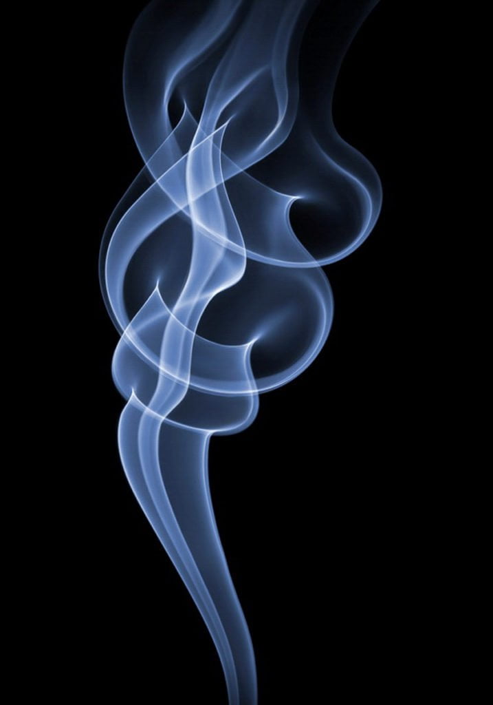


Ethereal forms shift and swirl in photographer Thomas Herbich’s series “Smoke”. The cigarette smoke in the images is a buoyant plume. As it rises, the smoke is sheared and shaped by its passage through the ambient air. What begins as a laminar plume is quickly disturbed, rolling up into vortices shaped like the scroll on the end of a violin. The vortices are a precursor to the turbulence that follows, mixing the smoke and ambient air so effectively that the smoke diffuses into invisibility. To see the full series, see Herbich’s website. (Image credits: T. Herbich; via Colossal; submitted by @jchawner, @__pj, and Larry B)
P.S. – FYFD now has a page listing all entries by topic, which should make it easier for everyone to find specific topics of interest. Check it out!

Supernova Explosion
Type 1a supernovae occur in binary star systems where a dense white dwarf star accretes matter from its companion star. As the dwarf star gains mass, it approaches the limit where electron degeneracy pressure can no longer oppose the gravitational force of its mass. Carbon fusion in the white dwarf ignites a flame front, creating isolated bubbles of burning fluid inside the star. As these bubbles burn, they rise due to buoyancy and are sheared and deformed by the neighboring matter. The animation above is a visualization of temperature from a simulation of one of these burning buoyant bubbles. After the initial ignition, instabilities form rapidly on the expanding flame front and it quickly becomes turbulent. (Image credit: A. Aspden and J. Bell; GIF credit: fruitsoftheweb, source video; via freshphotons)

Paint on Speakers
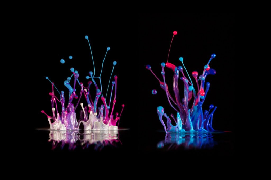
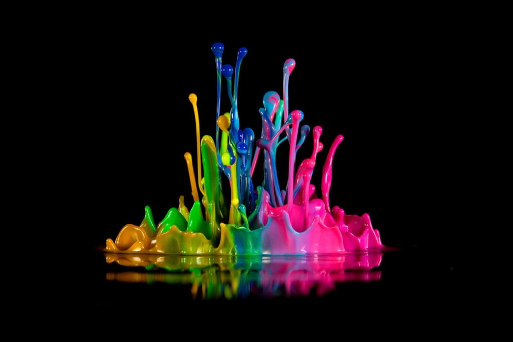
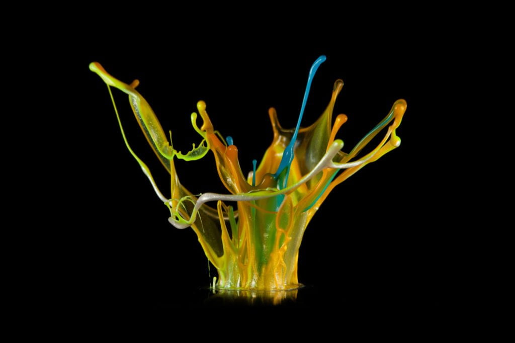


Paint seems to dance and leap when vibrated on a speaker. Propelled upward, the liquid stretches into thin sheets and thicker ligaments until surface tension can no longer hold the the fluid together and droplets erupt from the fountain. Often paints are shear-thinning, non-Newtonian fluids, meaning that their ability to resist deformation decreases as they are deformed. This behavior allows them to flow freely off a brush but then remain without running after application. In the context of vibration, though, shear-thinning properties cause the paint to jump and leap more readily. For more images, see photographer Linden Gledhill’s website. (Photo credit: L. Gledhill; submitted by pinfire)

4th Birthday: The Kaye Effect
Today’s post continues my retrospective on mind-boggling fluid dynamics in honor of FYFD’s birthday. This video on the Kaye effect was one of the earliest submissions I ever received–if you’re reading this, thanks, Belisle!–and it completely amazed me. Judging from the frequency with which it appears in my inbox, it’s delighted a lot of you guys as well. The Kaye effect is observed in shear-thinning, non-Newtonian fluids, like shampoo or dish soap, where viscosity decreases as the fluid is deformed. Like many viscous liquids, a falling stream of these fluids creates a heap. But, when a dimple forms on the heap, a drop in the local viscosity can cause the incoming fluid jet to slip off the heap and rebound upward. As demonstrated in the video, it’s even possible to create a stable Kaye effect cascade down an incline. (Video credit: D. Lohse et al.)

Measuring Wind Speed by Satellite
Weather modeling and forecasting in recent decades have benefited enormously from the availability of more data. For example, satellites now measure wind speeds over the open ocean, instead of data simply coming from isolated ships and buoys. The satellites do this by measuring the roughness of the ocean using radar or GPS signals bounced off the ocean surface. From this researchers can construct a map of wave height and direction like the one in the animation above. For a large body of water, waves are primarily generated by wind shearing the water at the interface. The waves we see are a result of the Kelvin-Helmholtz instability between the wind and ocean. Because this is a well-known behavior, it is possible to connect the waves we observe with the wind conditions that must have generated them. (Image credit: ESA; animation credit: Wired; submitted by jshoer)
Jupiter Timelapse
This timelapse video shows Jupiter as seen by Voyager 1. In it, each second corresponds to approximately 1 Jupiter day, or 10 Earth hours. Be sure to fullscreen it so that you can appreciate the details. The timelapse highlights the differences in velocity (and even flow direction!) between Jupiter’s cloud bands. It is these velocity differences that create the shear forces which cause Kelvin-Helmholtz instabilities–the series of overturning eddies–seen between the bands. Earth also has bands of winds moving in opposite directions, but there are fewer of them and the composition of our atmosphere is such that they do not make for such a dramatic naked eye view of large-scale fluid dynamics. (Video credit: NASA/JPL/B. Jónsson/I. Regan)
Kelvin-Helmholtz in the Lab
The Kelvin-Helmholtz instability looks like a series of overturning ocean waves and occurs between layers of fluids undergoing shear. This video has a great lab demo of the phenomenon, including the set-up prior to execution. When the tank is tilted, the denser dyed salt water flows left while the fresh water flows to the right. These opposing flow directions shear the interface between the two fluids, which, once a certain velocity is surpassed, generates an instability in the interface. Initially, this disturbance is much too small to be seen, but it grows at an exponential rate. This is why nothing appears to happen for many seconds after the tilt before the interface suddenly deforms, overturns, and mixes. In actuality, the unstable perturbation is present almost immediately after the tilt, but it takes time for the tiny disturbance to grow. The Kelvin-Helmholtz instability is often seen in clouds, both on Earth and on other planets, and it is also responsible for the shape of ocean waves. (Video credit: M. Hallworth and G. Worster)
Supercell Timelapse
The storm chasing group Basehunters captured this stunning timelapse of a supercell thunderstorm forming in Wyoming. This class of storm is characterized by the presence of a mesocyclone, seen here as a large, rotating cloud. These rotating features form when horizontal wind shear is redirected upright by an updraft. This requires a strong updraft, which is often formed by a capping inversion, where a layer of warm air traps colder air beneath it. Supercells can be very dangerous in their own right, releasing torrential rains and large hail, but they are also capable of spawning violent tornadoes. (Video credit: Basehunters; via Bad Astronomy; submitted by jshoer)
Why Ketchup is Hard to Pour
Oobleck gets a lot of attention for its non-intuitive viscous behaviors, but there are actually many non-Newtonian fluids we experience on a daily basis. Ketchup is an excellent example. Unlike oobleck, ketchup is a shear-thinning fluid, meaning that its viscosity decreases once it’s deformed. This is why it pours everywhere when you finally get it moving. Check out this great TED-Ed video for why exactly that’s the case. In the end, like many non-Newtonian fluids, the oddness of ketchup’s behavior comes down to the fact that it is a colloidal fluid, meaning that it consists of microscopic bits of a substance dispersed throughout another substance. This is also how blood, egg whites, and other non-Newtonian fluids get their properties. (Video credit: G. Zaidan/TED-Ed; via io9)