Today’s fastest boats use hydrofoils to lift most of a boat’s hull out of the water. This greatly reduces the drag a boat experiences, but it can also make the boat difficult to handle. One style of hydrofoil boat, called a single-track hydrofoil, uses two hydrofoils in line with one another to support and steer the boat. The pilot can steer the lead hydrofoil into the direction of a fall to correct it. Stability-wise, this is the same way that you keep a bicycle upright. On a boat, the situation is a bit tougher to manage, and, like riding a bike, it takes practice. A group of students published a full mathematical model for the dynamics of this kind of boat, which allows designers to test a prototype’s stability early in the design process and enables student teams to use computer simulators to train their pilots to drive a boat before putting them out on the water, similar to the way that airplane pilots train. (Image credit: TU Delft Solar Boat Team, source; research credit: G. van Marrewijk et al., pdf; via TU Delft News; submitted by Marc A.)
Tag: numerical simulation

Snowmelt
Much of the rain that falls on Earth began as snow high in the atmosphere. As it falls through warmer layers of air, the snowflakes melt and form water droplets. The details of this melting process have been difficult to capture experimentally, but a new computational model may provide insight. The basic process has a couple stages. As snow begins to melt, surface tension draws the water into concave areas nearby. When those regions fill up, the water flows out and merges with neighboring liquid, forming water droplets around a melting ice core.
Although this same sequence was observed for many types of snow, scientists also observed some important differences between rimed and unrimed snowflakes. Rime forms when supercooled water droplets freeze onto the surface of a snowflake. Lightly rimed snow still looks light and fluffy, like the animation above, but heavily rimed snow forms denser and more spherical chunks. Because there are lots of porous gaps in heavily rimed snow, water tends to gather there during initial melting. Rimed snow was also more likely to form one large water droplet rather than breaking into multiple droplets like snow with less rime. For more, check out NASA’s video and the Bad Astronomy write-up. (Image credit: NASA, source; research credit: J. Leinonen and A. von Lerber; via Bad Astronomy; submitted by Kam Yung-Soh)

Atmospheric Aerosols
Recently, NASA Goddard released a visualization of aerosols in the Atlantic region. The simulation uses real data from satellite imagery taken between August and October 2017 to seed a simulation of atmospheric physics. The color scales in the visualization show concentrations of three major aerosol particles: smoke (gray), sea salt (blue), and dust (brown). One of the interesting outcomes of the simulation is a visualization of the fall Atlantic hurricane season. The high winds from hurricanes help pick up sea salt from the ocean surface and throw it high in the atmosphere, making the hurricanes visible here. Fires in the western United States provide most of the smoke aerosols, whereas dust comes mostly from the Sahara. Tiny aerosol particles serve as a major nucleation source for water droplets, affecting both cloud formation and rainfall. With simulations like these, scientists hope to better understand how aerosols move in the atmosphere and how they affect our weather. (Image credit: NASA Goddard Research Center, source; submitted by Paul vdB)

Forming Craters


Asteroid impacts are a major force in shaping planetary bodies over the course of their geological history. As such, they receive a great deal of attention and study, often in the form of simulations like the one above. This simulation shows an impact in the Orientale basin of the moon, and if it looks somewhat fluid-like, there’s good reason for that. Impacts like these carry enormous energy, about 97% of which is dissipated as heat. That means temperatures in impact zones can reach 2000 degrees Celsius. The rest of the energy goes into deforming the impacted material. In simulations, those materials – be they rock or exotic ices – are usually modeled as Bingham fluids, a type of non-Newtonian fluid that only deforms after a certain amount of force is applied. An everyday example of such a fluid is toothpaste, which won’t extrude from its tube until you squeeze it.
The fluid dynamical similarities run more than skin-deep, though. For decades, researchers looked for ways to connect asteroid impacts with smaller scale ones, like solid impacts on granular materials or liquid-on-liquid impacts. Recently, though, a group found that liquid-on-granular impacts scale exactly the way that asteroid impacts do. Even the morphology of the craters mirror one another. The reason this works has to do with that energy dissipation mentioned above. As with asteroid impacts, most of the energy from a liquid drop impacting a granular material goes into something other than deforming the crater region. Instead of heat, the mechanism for dissipation here is the drop’s deformation. The results, however, are strikingly alike.
For more on how asteroid impacts affect the moon and other bodies, check out Emily Lakdawalla’s write-up, which also includes lots of amazing sketches by James Tuttle Keane, who illustrates the talks he hears at conferences! (Image credits: J. Keane and B. Johnson; via the Planetary Society; additional research and video credit: R. Zhao et al., source; submitted by jpshoer)

Lighting Engines
Combustion is complicated. You’ve ideally got turbulent flow, acoustic waves, and chemistry all happening at once. With so much going on, it’s a challenge to sort out the physics that makes one ignition attempt work while another fails. The animations here show a numerical simulation of combustion in a turbulent mixing layer. The grayscale indicates density contours of a hydrogen-air mixture. The top layer is moving left to right, and the lower layer moves right to left. This sets up some very turbulent mixing, visible in middle as multi-scale eddies turning over on one another.
Ignition starts near the center in each simulation, sending out a blast wave due to the sudden energy release. Flames are shown in yellow and red. As the flow catches fire, more blast waves appear and reflect. But while the combustion is sustained in the upper simulation, the flame is extinguished by turbulence in the lower one. This illustrates another challenge engineers face: turbulence is necessary to mix the fuel and oxidizer, but turbulence in the wrong place at the wrong time can put out an engine. (Image, research, and submission credit: J. Capecelatro, sources 1, 2)


Adaptive Meshing
The use of numerical simulations in fluid dynamics has exploded over the past half century with new computational techniques being developed constantly. Most methods involve solving the equations of motion (or an approximation thereof) on a grid of points known as a mesh. To accurately capture the physics, meshes must often be quite closely packed in areas where detail is needed, but they can be more widely spaced in areas where the flow is not changing quickly. An increasingly common technique is adaptive meshing in which the mesh of grid points shifts between time steps; this places more grid points where the flow requires them and removes them from less important areas in order to reduce computational time.
An example of adaptive meshing is shown above. On the left particles are falling into salt water. The colors show the concentration of particles. The right side shows the solid particles and the fluid mesh around them. Notice how the grid shifts as the particles fall. (Image credit: C. Jacobs et al., source)

How Cycling Position Affects Aerodynamics


New FYFD video! How much does a rider’s position on the bike affect the drag they experience? To find out I teamed up with folks from the University of Colorado at Boulder and at SimScale to explore this topic using high-speed video, flow visualization, and computational fluid dynamics.
Check out the full video below, and if you need some more cycling science before the Tour de France gets rolling, you can find some of my previous cycling-related posts here. (Image and video credit: N. Sharp; CFD simulation – A. Arafat)
ETA: Please note that the video contained in this post was sponsored by SimScale.

Simulating Thunderstorms
With today’s supercomputing power, it’s possible to simulate entire thunderstorms to study how and why some of them can spawn deadly tornadoes. The animation above comes from a computer simulation of a supercell thunderstorm. The simulation uses initial conditions from a 2011 storm that produced an EF-5 tornado – the highest category of tornado, based on its wind speeds. To see more of the simulation, check out the video below. One thing that might surprise you is just how enormous the towering supercell clouds are compared to the tornado produced in the simulation. Often what we can see of a storm from the ground is only the tiniest part of what goes into producing it. (Image credit: L. Orf et al., source; GIF via @popsci; video credit: UWSSEC)
Windy Urban Corridors (*)


For pedestrians, windy conditions can be uncomfortable or even downright dangerous. And while you might expect the buildings of an urban environment to protect people from the wind, that’s not always the case. The image above shows a simulation of ground-level wind conditions in Venice on a breezy day. While many areas, shown in blue and green, have lower wind speeds, there are a few areas, shown in red, where wind speeds are well above the day’s average. This enhancement often occurs in areas where buildings constrict airflow and funnel it together. The buildings create a form of the Venturi effect, where narrowing passages cause local pressure to drop, driving an increase in wind speed. Architects and urban designers are increasingly turning to numerical simulations and CFD to study these effects in urban environments and to search for ways to mitigate problems and keep pedestrians safe. (Image credits: CFD analysis – SimScale; pedestrians – Saltysalt, skolnv)
(*) This post was sponsored by SimScale, the cloud-based simulation platform. SimScale offers a free Community plan for anyone interested in trying CFD, FEA and thermal simulations in their browser. Sign up for a free account here.
For information on FYFD’s sponsored post policy, click here.

Creating Moana’s Ocean
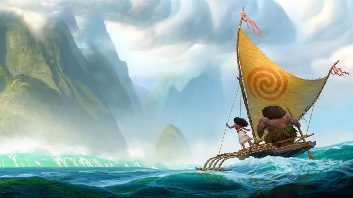


Hopefully by now you’ve had an opportunity to see Disney’s film Moana. Fluid dynamics play a central role in the movie, and Disney’s animators faced the challenge of hundreds of shots requiring special effects to animate water, lava, waves, and wind. Science Friday has a great segment interviewing a couple of Moana’s animators, in which they discuss the process of turning the ocean itself into a character.
Because the physics of fluids is so complex, scientists and animators differ in the way they approach simulations. Scientists usually try to capture a full physical representation of a flow, simulating every detail to the smallest scale and time step. Animators, on the other hand, are interested in capturing a realistic feel for a flow. For an animator, the simulation should be exactly as complex as necessary to make the water move in a way a person believes it should. With Moana, animators had the extra challenge of melding the ocean character’s actions with appropriate water physics–think bubbles, drops, and splashes. The results are impressive and exceptionally fun. (Image credits: Disney/Science Friday; via Jesse C.)