One of the common themes in aerodynamics, especially in sports applications, is that tripping the flow to turbulence can decrease drag compared to maintaining laminar flow. This seems counterintuitive, but only because part of the story is missing. When a fluid flows around a complex shape, there are actually three options: laminar, turbulent, or separated flow. An object’s shape creates pressure forces on the surrounding fluid flow, in some cases causing an increasing, or unfavorable, pressure gradient. When this occurs, fluid, especially the slower-moving fluid near a surface, can struggle to continue flowing in the streamwise flow direction. Consider the video above, in which the flow moves from left to right. Near the surface a turbulent boundary layer is visible, where fluid motion is significantly slower and more random. Occasionally the flow even reverses direction and billows up off the surface. This is separation. Unlike laminar boundary layers, turbulent boundary layers can better resist and recover from flow separation. This is ultimately what makes them preferable when dealing with the aerodynamics of complex objects. (Video credit: A. Hoque)
Search results for: “turbulence”

The Structure of Turbulence
Though they may appear random at first glance, turbulent flows do possess structure. The video above shows a numerical simulation of a mixing layer, a flow in which two adjacent regions of fluid move with different velocities. The upper third of the frame shows a top view, and the bottom frame shows a side view, in which the upper fluid layer moves faster than the lower one. The difference in velocities creates shear which quickly drives the mixing layer into turbulence. But watch the chaos carefully, and your eye will pick out vortices rolling clockwise in the largest scales of the mixing layer. These features are known as coherent structures, and they are key to current efforts to understand and model turbulent flows. (Video credit: A. McMullan)

Turbulence and Magnetic Field Lines
During a solar flare, magnetic field lines on the sun are often visible due to the flow of plasma–charged particles–along the lines. According to theory, these magnetic lines should remain intact, but they are sometimes observed breaking and reconnecting with other lines. An interdisciplinary team of researchers suggests that turbulence may be the missing link. In their magnetohydrodynamic simulation, they found that the presence of chaotic turbulent motions made the magnetic line motion entirely unpredictable, whereas laminar flows behaved according to conventional flux-freezing theory. (Photo credit: NASA SDO; Research credit: G. Eyink et al.; via SpaceRef; submitted by jshoer)

Simulated Turbulence
This image, taken from a direct numerical simulation, shows turbulence in a stably stratified flow in which lighter fluid sits atop a denser fluid. In the image lighter colors represent denser fluid. Turbulence is created by the shear forces caused when the lighter fluid on top moves faster than the denser fluid on the bottom; however the stable stratification will tend to counteract or stabilize the turbulence. Note the vast variety and detail of the scales involved in turbulence; this is what makes it such a difficult process to simulate and model. (Image credit: G. Matheou and D. Chung, NASA/JPL-Caltech)

Structures in Turbulence
Despite its appearance, there is order in the chaos of turbulence. These snapshots from a turbulent channel flow simulation outline these coherent structures in black. The top photo shows a top view looking down on the channel and the bottom image shows a side view of the channel. It is thought that studying these coherent structures may help shed light on turbulence and its formation, which remains one of the great open questions of classical physics. (Photo credit: M. Green)

Transition to Turbulence
Smoke introduced into the boundary layer of a cone rotating in a stream highlights the transition from laminar to turbulent flow. On the left side of the picture, the boundary layer is uniform and steady, i.e. laminar, until environmental disturbances cause the formation of spiral vortices. These vortices remain stable until further growing disturbances cause them to develop a lacy structure, which soon breaks down into fully turbulent flow. Understanding the underlying physics of these disturbances and their growth is part of the field of stability and transition in fluid mechanics. (Photo credit: R. Kobayashi, Y. Kohama, and M. Kurosawa; taken from Van Dyke’s An Album of Fluid Motion)
Simulating Turbulence
Turbulent flows are complicated to simulate because of their many scales. The largest eddies in a flow, where energy is generated, can be of the order of meters, while the smallest scales, where energy is dissipated, are of the order of fractions of a millimeter. In Direct Numerical Simulation (DNS), the exact equations governing the flow are solved at all of those scales for every time step–requiring hundreds or thousands of computational hours on supercomputers to solve even a small domain’s worth of flow, as on the airplane wing in the video. Large Eddy Simulation (LES) is another technique that is less computationally expensive; it calculates the larger scales exactly and models the smaller ones. The video shows just how complicated the flow field can look. The red-orange curls seen in much of the flow are hairpin vortices, named for their shape, and commonly found in turbulent boundary layers.

Volcanic Turbulence
One of the characteristics of turbulence is its large range of lengthscales. Consider the ash plume from this Japanese volcano. Some of the eddy structures are tens, if not hundreds, of meters in size, yet there is also coherence down to the scale of centimeters. In turbulence, energy cascades from these very large scales to scales small enough that viscosity can dissipate it. This is one of the great challenges in directly calculating or even simply modeling turbulence because no lengthscale can be ignore without affecting the accuracy of the results. #

Turbulence Near the Wall
This photo shows a flow visualization of a turbulent boundary layer at Mach 2.8. The direction of flow is from right to left. In nature, the boundary layer between a surface and a fluid is usually turbulent but impossible to see. The visualization represents an instantaneous snapshot of the flow. Turbulence is known for its intermittency–its strong variation in time–a characteristic that is clear just from comparing the two snapsnots. #
“Inferno”


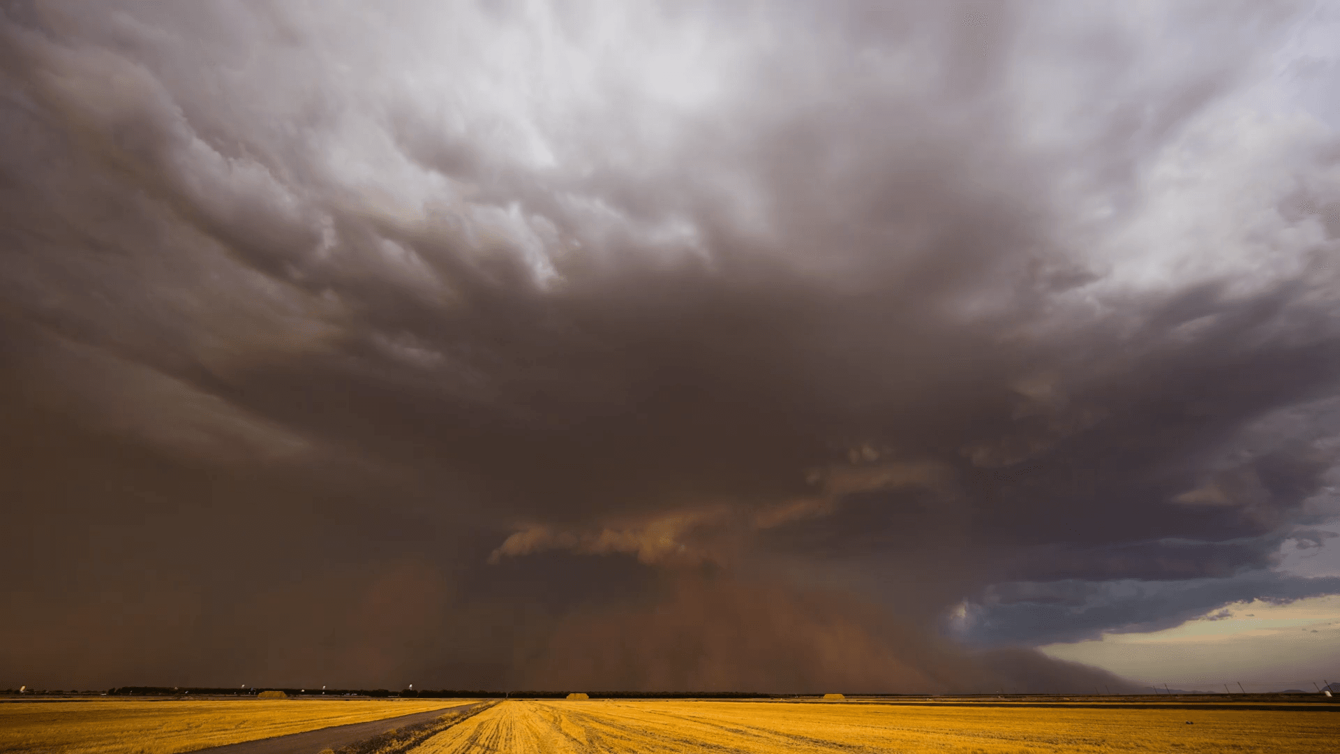
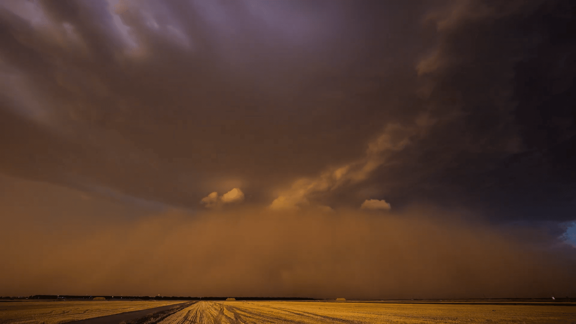
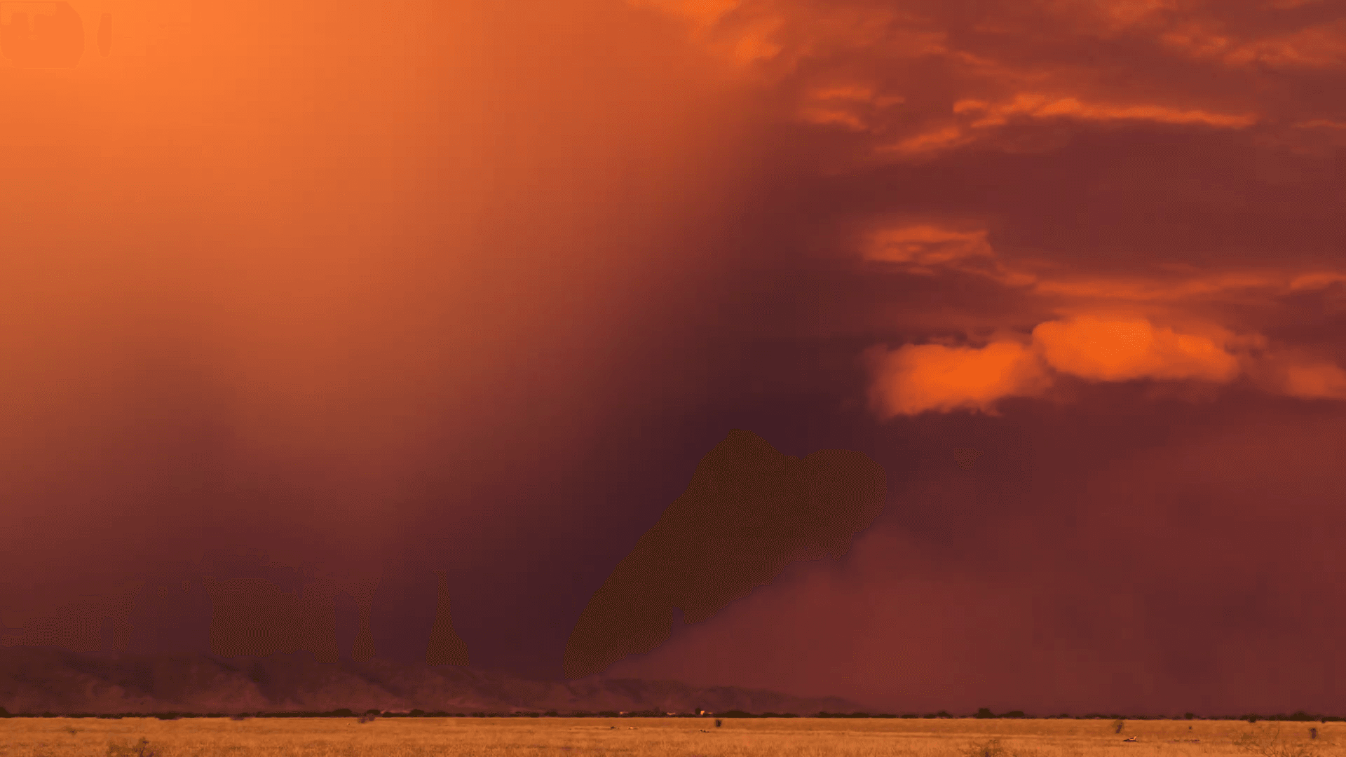
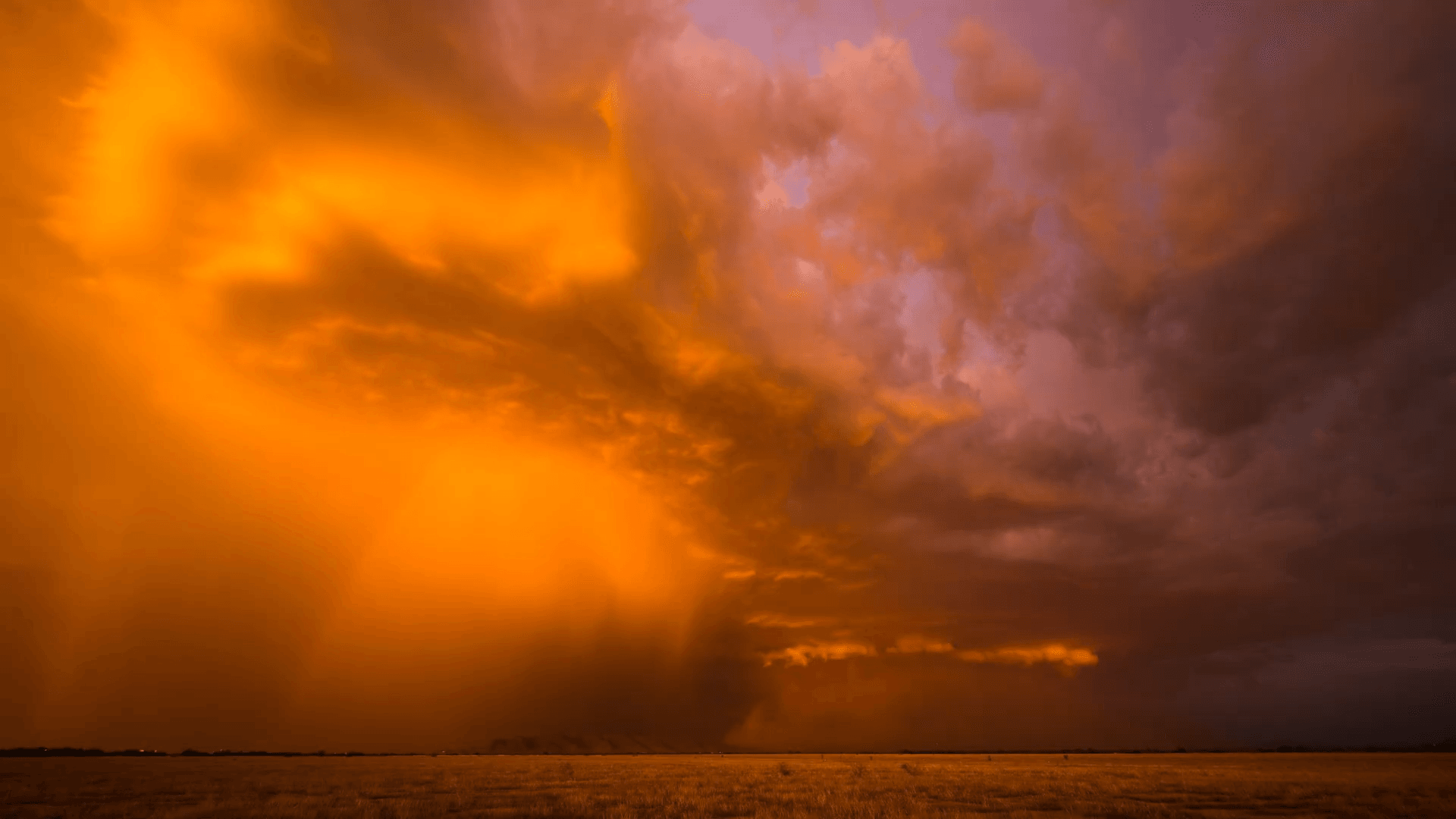
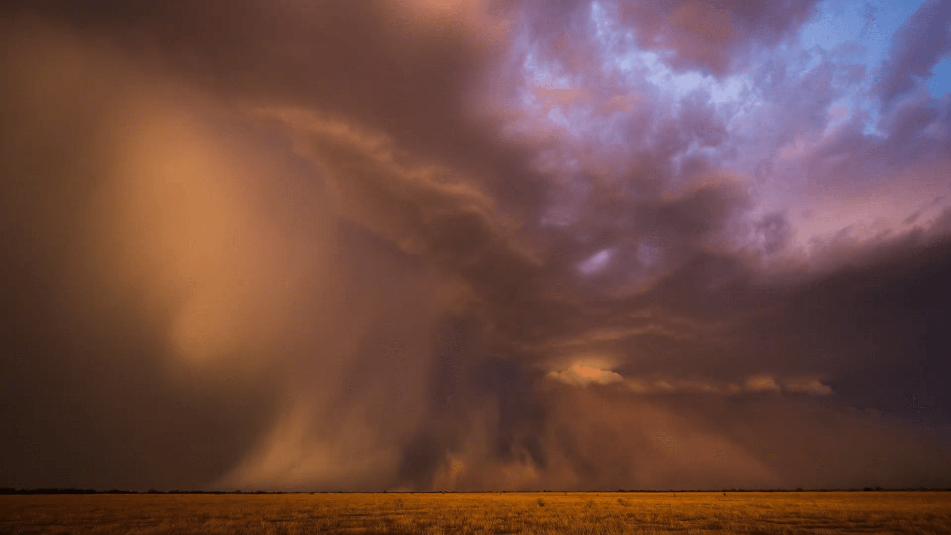
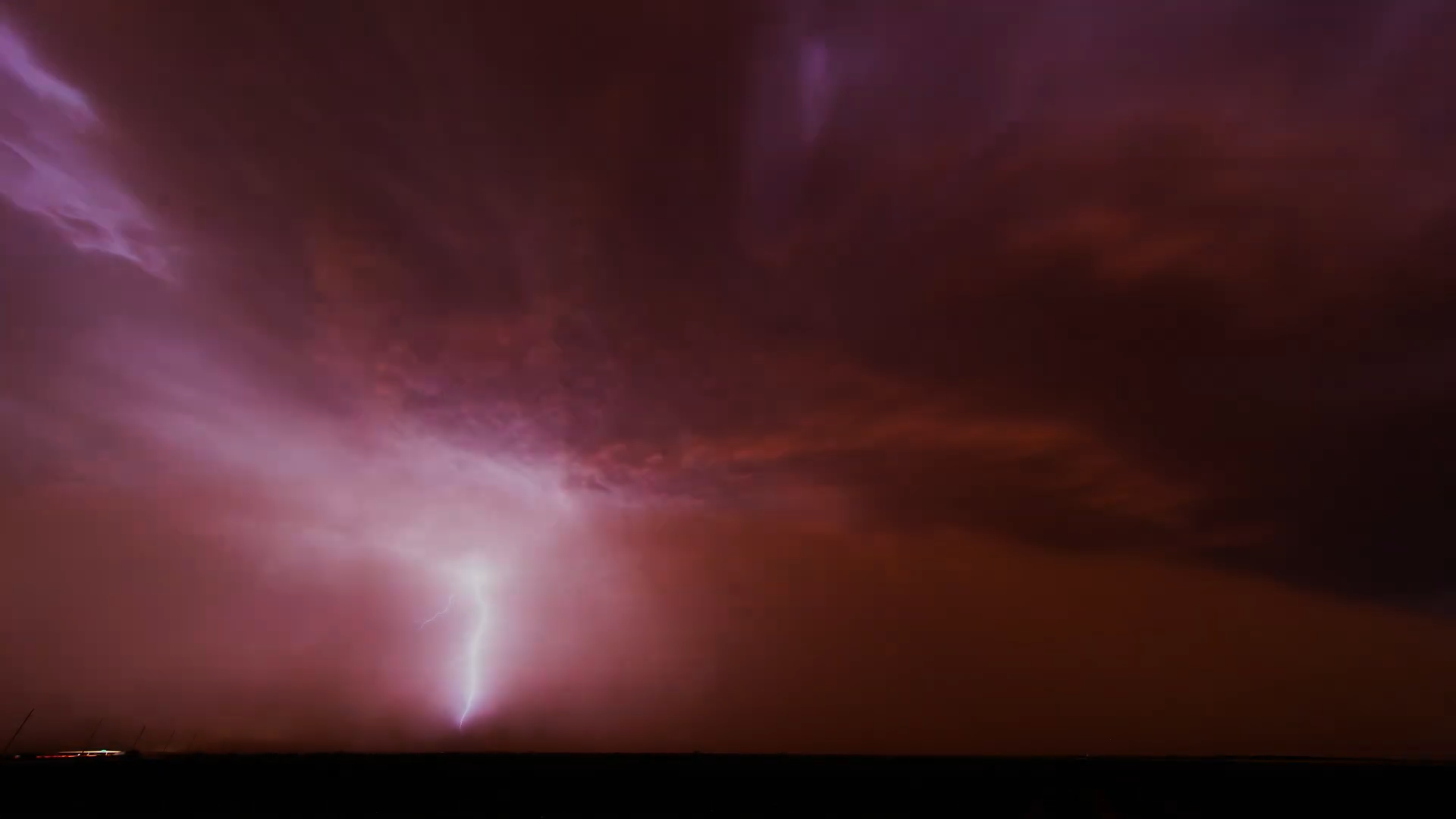
Nothing showcases the incredible power of our atmosphere like storms, and no one does stormchase photography like Mike Olbinski. In this vignette, he shows a stunning line of supercells caught near sunset on July 17, 2022. The high shear–combined with the setting sun–put on an incredible show. Dust blown up in a haboob, microbursts and downpours in the distance, and lots of churning, roiling turbulence. (Video and image credit: M. Olbinski)
Fediverse Reactions
-