
Efficient mixing of fluids is vital for many applications, including fuel injection for all types of combustion and masking the exhaust of stealth fighters. Star-shaped lobed nozzles can produce jets that mix more effectively than conventional jets. This photo shows cross-sections of the jet at several downstream distances from the nozzle exit. (Photo credit: H. Hu et al)
Tag: turbulence

Separation and Stall
This flow visualization of a pitching wind turbine blade demonstrates why lift and drag can change so drastically with angle of attack. When the angle the blade makes with the freestream is small, flow stays attached around the top and bottom surfaces of the blade. At large (positive or negative) angles of attack, the flow separates from the turbine blade, beginning at the trailing edge and moving forward as the angle of attack increases. The separated flow appears as a region of recirculation and turbulence. This is the same mechanism responsible for stall in aircraft. (Submitted by Bobby E)

Structures in Turbulence
Despite its appearance, there is order in the chaos of turbulence. These snapshots from a turbulent channel flow simulation outline these coherent structures in black. The top photo shows a top view looking down on the channel and the bottom image shows a side view of the channel. It is thought that studying these coherent structures may help shed light on turbulence and its formation, which remains one of the great open questions of classical physics. (Photo credit: M. Green)

Ink Sculptures

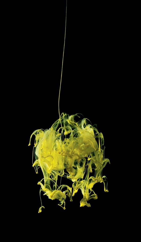
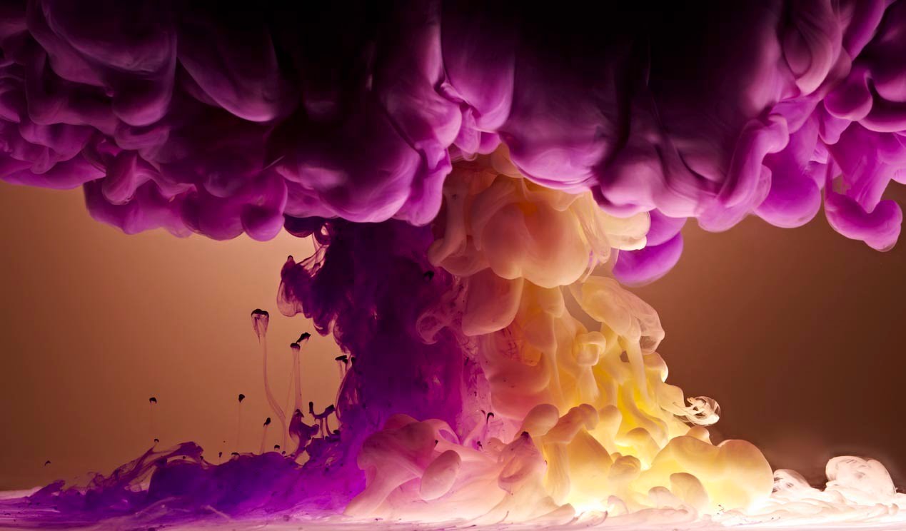
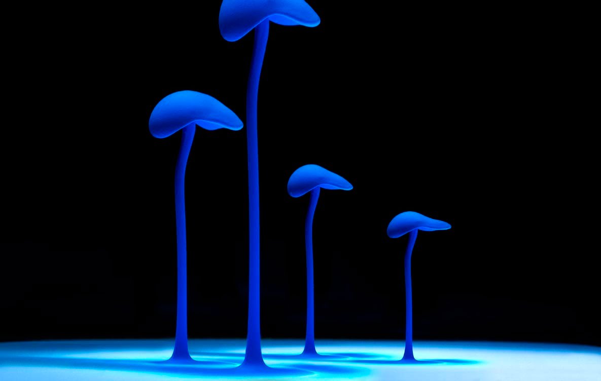
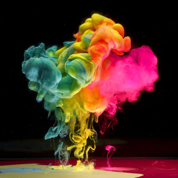
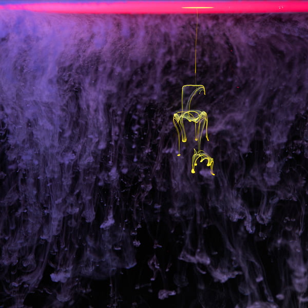
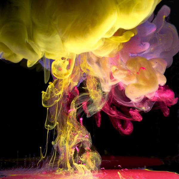
Dripping ink into water can create fantastic structures as the two fluids mix. In this artwork there are numerous complex mixing phenomena: the eddies and multiple scales of turbulence; the long, thin streams of laminar flow; and the wispy mushrooms and umbrellas of the Rayleigh-Taylor instability. (Photo credit: Mark Mawson; via @thinkgeek)
Underwater Plumes
During 2010’s Deepwater Horizon oil spill there were reports of underwater plumes of oil escaping collection. This video demonstrates how such a plume can form. There are two clips shown here; in both the tank is filled with salt water of varying salinity, with denser saltwater at the bottom. The first jet is a green alcohol/water mixture and the second is a red gauge oil. Both jets have the same density and flow rate, but they vary in their Reynolds number. The first turbulent jet gets trapped at the interface between the denser and lighter saltwater while the less turbulent red jet passes the interface with no difficulty. The researchers suggest that strong turbulence can create an emulsion, a mixture of two normally immiscible fluids–imagine shaking a container of oil and vinegar really well–which can lead to underwater trapping.

Transition to Turbulence
Smoke introduced into the boundary layer of a cone rotating in a stream highlights the transition from laminar to turbulent flow. On the left side of the picture, the boundary layer is uniform and steady, i.e. laminar, until environmental disturbances cause the formation of spiral vortices. These vortices remain stable until further growing disturbances cause them to develop a lacy structure, which soon breaks down into fully turbulent flow. Understanding the underlying physics of these disturbances and their growth is part of the field of stability and transition in fluid mechanics. (Photo credit: R. Kobayashi, Y. Kohama, and M. Kurosawa; taken from Van Dyke’s An Album of Fluid Motion)
Jellyfish Flow
Florescent dye reveals the flow pattern of ocean water around a swimming jellyfish. Some researchers posit that fluid drift associated with the swimming of marine animals may be as substantial a factor in ocean mixing as turbulence caused by the wind and tides. If true, modeling of climate change–past, present, and future–would need to take into account the biology of the ocean as well! #

Jovian Storms


Home to storms capable of lasting for a hundred years or more, Jupiter’s atmosphere is a highly turbulent place. Currently, no comprehensive theory exists to explain the symmetry of Jupiter’s bands of clouds and the persistence of vortices such as the Great Red Spot, however, the mixing and stratification visible on the planet remains a beautiful reminder of the power of fluid dynamics. (Photo credits:Cassini – 1, 2, Voyager 1, New Horizons – 1, 2)
Smoke Transition
Smoke issuing from a round jet undergoes transition from laminar to turbulent flow. As the smoke moves past the unmoving ambient air, the friction between these two layers creates shear and triggers a Kelvin-Helmholtz instability, recognizable by the formation and roll up of vortices along the edges of the jet. Those vortices then roll together in pairs, detach, and devolve into a generally turbulent flow. Because turbulence is far more efficient at mixing than a laminar flow is, the smoke seems to disappear.
Coughing Contagions
Schlieren imaging has applications even in public health. This video demonstrates the spread of contagion via coughing with and without a mask on. Although air from the cougher’s lungs escapes the sides of the mask, it mostly rises on a thermal plume rather than projecting 1 to 2 meters forward in a turbulent jet as in the maskless case. Flu season is just starting. Don’t forget to get your flu shot!


