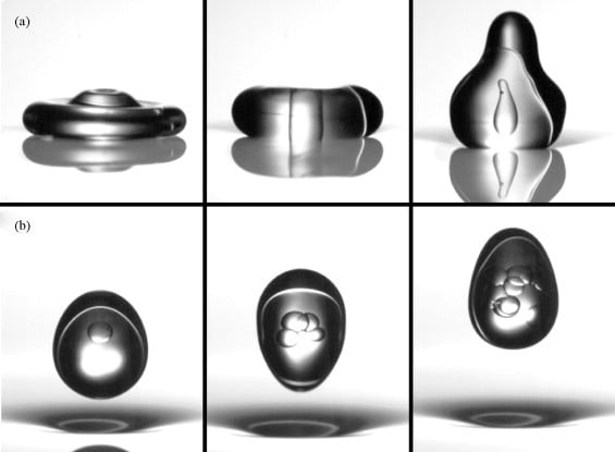
Mixing immiscible liquids–like oil and water–is tough. The best one can usually do is create an emulsion, in which droplets of one fluid are suspended in another. The series of images above shows a double emulsion consisting of oil and water that’s been formed by bouncing the compound droplet on a vibrating bath. The vibration of the liquid surface keeps the droplet from coalescing with the bath and the deformation provides mixing. The top row shows the initial impact while the bottom row of images shows the droplet after many bounces. As time goes on, the layer of oil around the compound drop becomes a cluster of tiny droplets contained within the water portion of the drop. (Photo credit: D. Terwagne et al.)
Tag: mixing

Mixing the Southern Ocean
Motion in the ocean is driven by many factors, including temperature, salinity, geography, and atmospheric interactions. While global currents dictate much of the large-scale motion, it’s sometimes the smaller scales that impact the climate. This visualization shows numerically simulated data from the Southern Ocean over the course of a year. The eddies that swirl off from the main currents are responsible for much of the mixing that occurs between areas of different temperature, which ultimately impacts large-scale temperature distributions, in this case affecting the flux of heat toward Antarctica. (Video credit: I. Rosso, A. Klocker, A. Hogg, S. Ramsden; submitted by S. Ramsden)
Mixing While Laminar
Although turbulent flows are known for their mixing efficiency, in manufacturing there can often be a need to mix laminar fluid streams without the increased shear stress of a turbulent flow. This can be particularly important for polymeric liquids, where too much shear stress could damage the polymer chains. One possibility is using a static mixer, such as the one demonstrated in this video, which, when placed in pipe flow, will deflect the pipe’s contents in such a way as to produce efficient mixing over a short distance. Here two streams of high-viscosity epoxy are mixed through such a static mixer, hardened, and then ground to show the mixing at each level of the static mixer. (Video credit: Sulzer)
Inside a Blender
The fluid dynamics of a commercial-quality blender amount to a lot more than just stirring. Here high-speed video shows how the blender’s moving blades create a suction effect that pulls contents down through the middle of the blender, then flings them outward. This motion creates large shear stresses, which help break up the food, as well as turbulence that can mix it. But if you watch carefully, you’ll also see tiny bubbles spinning off the blades. These bubbles, formed by the pressure drop of fluid accelerated over the arms of the blades, are cavitation bubbles. When they collapse, or implode, they create localized shock waves that further break up the blender’s contents. This same effect is responsible for damage to boat propellers and lets you destroy glass bottles. (Video credit: ChefSteps; via Wired; submitted by jshoer)
Ink Drops
This super high resolution video (check the original on YouTube) by filmmaker Jacob Schwarz features slow motion diffusion of ink into water. The subtle differences in density between the ink and the water promote instabilities such as the Rayleigh-Taylor instability and its distinctive cascade of mushroom- or umbrella-like shapes. The mixing of two fluids seems like a simple concept, but the reality is beautiful, complex, and always fascinating. (Video credit: J. Schwarz; submitted by Rebecca S.)

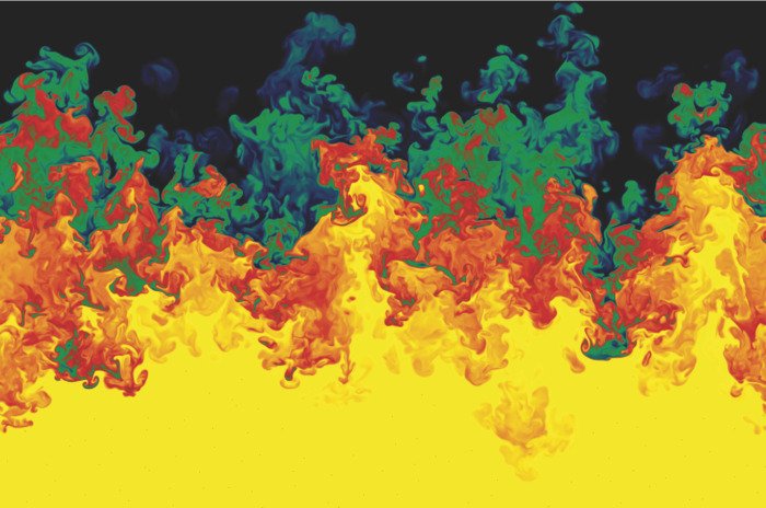
Mixing Physics
When a dense fluid sits above a lighter fluid in a gravitational field, the interface between the two fluids is unstable. It breaks down via a Rayleigh-Taylor instability, with mushroom-like protrusions of the lighter fluid into the heavier one. The image above comes from a numerical simulation of this effect well after the initial instability; the darker colors represent denser fluids and lighter colors are less dense fluids. The flow here has progressed to turbulence, and the authors of the simulation are exploring the statistical nature of this flow breakdown relative to the classical case of isotropic, homogeneous turbulence. (Photo credit: W. Cabot and Y. Zhou)

Phytoplankton and Sediments
Pale sediments are carried out to sea by the rivers of the Mergui Archipelago of Myanmar. Dark blue ocean waters mix with the sediment, creating turbulent swirls in this natural color satellite image. With the sediment comes valuable nutrients for plant life in the ocean, which can prompt the formation of phytoplankton blooms. (Photo credit: Michael Taylor/Landsat/NASA)
Mixing Physics
One of the most commonly observed fluid instabilities is the Rayleigh-Taylor instability, which occurs between fluids of differing densities. It’s most often seen when a denser fluid sits over a lower density fluid. In the video above, this is demonstrated experimentally: a lower density green fluid mixes in with the clear, higher density fluid. This is the classical case in which each initial region of fluid is uniform in density prior to the removal of the barrier. But what happens when each zone has its own variation in density? This is the second case. Before the barrier is removed, each region of the tank has a varying–or stratified–fluid density. In this case, the unmixed fluids are stably stratified, meaning that the fluid density increases with depth. At the barrier interface, the two separate fluids are still unstably stratified–with the denser fluid on top–so when the barrier is removed, the Rayleigh-Taylor instability still drives their mixing. Because of the stable stratification within the original unmixed fluids, the mixing region after the barrier’s removal is more limited. (Video credit: M. D. Wykes and S. B. Dalziel; via PhysicsCentral by APS)
Stirring Faces
This video features simulation of the laminar flow around a plate plunging sinusoidally in a quiescent flow. As the plate moves up and down, it mixes the fluid around it. This is visualized in several ways, beginning with the vorticity. Clockwise and anti-clockwise vortices are shed by the edges of the plate as it moves. The flow is also visualized using particle trajectories, which are classified by their tendency to accumulate (attract) or lose (repel) particles. These trajectories are particularly intriguing to watch develop as they appear to show ornate faces and designs. (Video credit: S. L. Brunton and C. W. Rowley)

The Beauty of the Great Red Spot

Jupiter is home to one of the most famous storms in the solar system, the Great Red Spot, which Earth observations place at a minimum of 180 (Earth) years in duration. Some evidence suggests that it may have been observed by humans as early as 1665. The magnitude of such a storm is almost unimaginable. At its narrowest point, the storm is still as wide as our entire planet and observations from the Voyager crafts indicate that the storm has 250 mph winds. The scale of mixing and turbulence around the storm, seen in photographs, is stunning and beautiful. (Photo credits: NASA/Voyager 1 and Michael Benson; submitted by oneheadtoanother)