In experiments, it can be difficult to track individual fluid structures as they flow downstream. Here researchers capture this spatial development by towing a 5-meter flat plate past a stationary camera while visualizing the boundary layer – the area close to the plate. The result is that we see turbulent eddies evolving as they advect downstream. Despite the complicated and seemingly chaotic flow field, the eye is able to pick out patterns and structure, like the merging of vortices that lifts eddies up into turbulent bulges and the entrainment of freestream fluid into the boundary layer as the eddies turn over or collapse. It is also a great demonstration of how the Reynolds number relates to the separation of scales in a turbulent flow. Notice how much richer the variety of length-scale is for the higher Reynolds number case and how thoroughly this mixes the boundary layer. (Video credit: J. H. Lee et al.)
Tag: flow visualization

Wake Vortices at Night
The ends of an airplane’s wings generate vortices that stretch back in the wake of the plane. Most of the time these vortices are invisible, even if their effects on lift are distinctive. Here an A-340 coming in for a foggy landing demonstrates the size and strength of these vortices. Notice how the fog gets swept up and away by the vortices. Pilots will sometimes use this effect to their advantage in clearing a runway of fog by making repeated low-passes to clear the fog before landing. (Video credit: A. Ruesch; submitted by Jens F.)

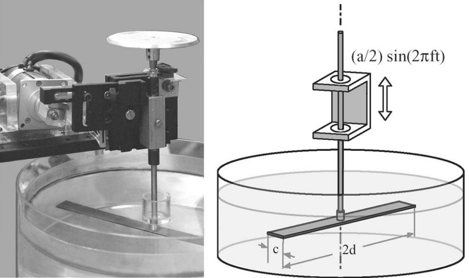
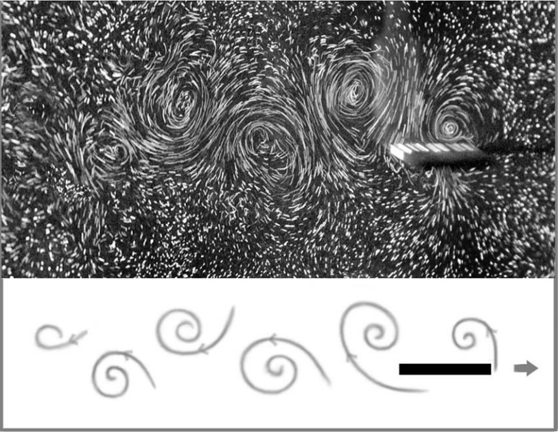
Imitating Flapping Flight

Flapping flight, despite being utilized by creatures of many sizes in nature, remains remarkably difficult to engineer. In this experiment, a simple rectangular wing is flapped up and down sinusoidally. Above a critical flapping frequency, the wing–which is free to rotate–accelerates from rest to a constant speed. This rotation is equivalent to forward flight. The upper image shows a photo and schematic of the setup, while the lower images shows flow visualization of the wing’s wake. The wing moves to the right, shedding thrust-providing periodic vortices in its wake. (Photo credits: N. Vandenberge et al.)
Mixing the Southern Ocean
Motion in the ocean is driven by many factors, including temperature, salinity, geography, and atmospheric interactions. While global currents dictate much of the large-scale motion, it’s sometimes the smaller scales that impact the climate. This visualization shows numerically simulated data from the Southern Ocean over the course of a year. The eddies that swirl off from the main currents are responsible for much of the mixing that occurs between areas of different temperature, which ultimately impacts large-scale temperature distributions, in this case affecting the flux of heat toward Antarctica. (Video credit: I. Rosso, A. Klocker, A. Hogg, S. Ramsden; submitted by S. Ramsden)

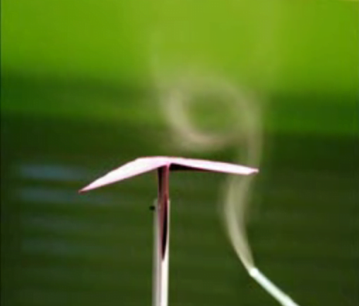
Lift on a Paper Plane
In this still image from a student experiment, smoke visualization shows the formation of a vortex over the wing of a paper airplane during a wind tunnel test. This wing vortex is mirrored on the opposite wing, though there is no smoke to show it. At high angle of attack, the delta-wing shape of the traditional paper air plane creates these vortices on the upper surface, which helps generate the lift necessary to keep the plane aloft. (Photo credit: A. Lindholdt, R. Frausing, C. Rechter, and S. Rytman)

Shock Waves in Flight
Schlieren photography allows visualization of density gradients, such as the sharp ones created by shock waves off this T-38 aircraft flying at Mach 1.1 around 13,000 ft. Although shock waves are relatively weak at this low supersonic Mach number, they persist, as seen in the image, at significant distances from the craft. The sonic boom associated with the passage of such a vehicle overhead is due to the pressure change across a shock wave. The higher the altitude of the supersonic craft, the less intense its shock wave, and thus sonic boom, will be by the time it reaches ground level. (Photo credit: NASA)

Humpback-Inspired Turbine Blades

The bumps–or tubercles–on the edge of a humpback whale’s fins have important hydrodynamic effects on its swimming. Here dye is used to visualize flow over a hydrofoil with tubercle-like protuberances–a sort of artificial whale fin. Dye released from the peaks and troughs of the protuberances flows straight back in a narrow line before breakdown to turbulence. But the dye released from ports on the shoulders of the protuberances twists and spirals into vortices. At angle of attack, these vortices are stronger. They may help keep flow from separating on the upper side of a whale’s fin. (Photo credits: SIDwilliams, H. Johari)
Spin-Up
With the Oscars just over, it seems like a good time for some movie-trailer-style fluid dynamics. This video shows a rotating water tank from the perspective of a camera rotating with the tank at 10 rpm. Initially, the tank and its contents are at rest. When the tank begins spinning, the fluid inside responds. Pink potassium permanganate crystals at the bottom of the tank show fluid motion as they dissolve, and food coloring is spread on the water’s surface to show motion there. Fluid near the edge of the tank reaches the tank’s rotational velocity fastest, due to friction with the wall, while fluid near the center of the tank takes longer to spin up to speed. This creates the spiral-galaxy-like shape in the dye. Eventually viscosity will transmit the effects of the wall’s motion even into the center of the tank. (Video credit: UCLA Spinlab)

Dye Flow
Fluid flow near a surface–inside the boundary layer–can often be unstable. This image shows one possible instability, formed when a cylinder is rotated back and forth about its longitudinal axis. This oscillation and the curvature of the cylinder destabilize flow in the boundary layer, forming vortices that line the cylinder. This particular behavior is called a Görtler instability. To visualize it, threads soaked in fluorescing dye have been embedded into slits in the cylinder. The cylinder is oscillated in a water tank and ultraviolet light is used to fluoresce the dye for the image. (Photo credit: Miguel Canals/University of Hawaii)
Laser-Induced Fluorescence
As demonstrated in the video above, lasers can be used to excite molecules into a higher energy state, which will decay via the emission of photons, causing the medium to glow. This laser-induced fluorescence is utilized in several techniques for measurements in fluid dynamics, including planar laser-induced fluorescence (PLIF) and molecular tagging velocimetry (MTV). In these techniques a flow is usually seeded with a fluorescing material–nitric oxide is popular for super- and hypersonic flows–and then lasers are used to excite a slice of the flow field. The resulting fluorescence can be used for both qualitative and quantitative flow measurements. Here are a couple of examples, one in low-Reynolds number flow and one in combustion. (Video credit: L. Martin et al./UC Berkeley)