With today’s supercomputing power, it’s possible to simulate entire thunderstorms to study how and why some of them can spawn deadly tornadoes. The animation above comes from a computer simulation of a supercell thunderstorm. The simulation uses initial conditions from a 2011 storm that produced an EF-5 tornado – the highest category of tornado, based on its wind speeds. To see more of the simulation, check out the video below. One thing that might surprise you is just how enormous the towering supercell clouds are compared to the tornado produced in the simulation. Often what we can see of a storm from the ground is only the tiniest part of what goes into producing it. (Image credit: L. Orf et al., source; GIF via @popsci; video credit: UWSSEC)
Tag: computational fluid dynamics

Creating Moana’s Ocean

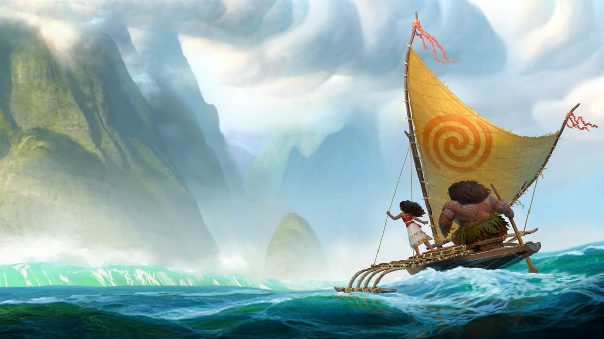


Hopefully by now you’ve had an opportunity to see Disney’s film Moana. Fluid dynamics play a central role in the movie, and Disney’s animators faced the challenge of hundreds of shots requiring special effects to animate water, lava, waves, and wind. Science Friday has a great segment interviewing a couple of Moana’s animators, in which they discuss the process of turning the ocean itself into a character.
Because the physics of fluids is so complex, scientists and animators differ in the way they approach simulations. Scientists usually try to capture a full physical representation of a flow, simulating every detail to the smallest scale and time step. Animators, on the other hand, are interested in capturing a realistic feel for a flow. For an animator, the simulation should be exactly as complex as necessary to make the water move in a way a person believes it should. With Moana, animators had the extra challenge of melding the ocean character’s actions with appropriate water physics–think bubbles, drops, and splashes. The results are impressive and exceptionally fun. (Image credits: Disney/Science Friday; via Jesse C.)

Simulating the Earth
Computational fluid dynamics and supercomputing are increasingly powerful tools for tracking and understanding the complex dynamics of our planet. The videos above and below are NASA visualizations of carbon dioxide in Earth’s atmosphere over the course of a full year. They are constructed by taking real-world measurements of atmospheric conditions and carbon emissions and feeding them into a computational model that simulates the physics of our planet’s oceans and atmosphere. The result is a visualization of where and how carbon dioxide moves around our planet.
There are distinctive patterns that emerge in a visualization like this. Because the Northern Hemisphere contains more landmass and more countries emitting carbon, it contains the highest concentrations of carbon dioxide, but winds move those emissions far from their source. As seasons change and plants begin photosynthesizing in the Northern Hemisphere, concentrations of carbon dioxide decrease as plants take it up. When the seasons change again, that carbon is re-released.
These visualizations underscore the fact that these carbon emissions impact everyone on our planet–nature does not recognize political borders–and so we share a joint responsibility in whatever actions we take. (Video credit: NASA Goddard; h/t to Chris for the second vid)

A Molecular View of Boiling
All matter is made up of molecules. But most of the time we treat fluids as materials with given properties – like density, viscosity, and surface tension – without worrying about the individual molecules responsible for those material characteristics. Now that we have much more powerful computers, though, we can begin to simulate fluid behavior in terms of molecules.
The animations above show some examples of this. In the top animation, we see a gas condensing into a liquid. As the temperature decreases, molecules start clumping together, and eventually settle into a droplet on the solid surface. The lower animation shows the opposite situation – boiling – in which bubbles of vapor nucleate next to the solid surface and grow as more liquid changes phase. To see more examples, including droplets pinching off, check out the full video. (Image credit: E. Smith et al., source; submitted by O. Matar)

Amphibious Adaptation
Every year newts move to the water in the springtime to mate before returning to land for the rest of the year. This annual aquatic relocation is accompanied by changes in the newt’s body. Flaps of skin grow from their upper jaw to their lower jaw, partially closing their mouths at the corners. This can be seen in the left column of the animation compared to the center and right.
Numerical simulation shows that this mouth change has a significant impact on the newt’s ability to hunt underwater. Newts are suction feeders, who open their jaws and expand their mouth cavity to suck in water and their prey. By closing off the corners of their mouths during their aquatic phase, the newts generate more suction, reaching peak flow velocities 10% to 50% higher than in their terrestrial form and enabling them to pull prey from 15% further away. When they leave the water, the newts lose the extra flaps so that their mouths can open wider for catching prey on land. (Image credit: S. Van Wassenbergh and E. Heiss, source)

Turbulence in the Solar Wind
One of the key features of turbulent flows is that they contain many different length scales. Look at the plume from an erupting volcano, and you’ll see eddies that are hundreds of meters across as well as tiny ones on the order of millimeters. This enormous difference in scale is one of the major challenges in simulating turbulent flows. Since energy enters at the large scale and is passed to smaller and smaller scales before being dissipated at the tiniest scales of the flow, properly simulating a turbulent flow requires resolving all of these length scales. This is especially challenging for applications like the solar wind – the stream of charged particles that flows from the sun and gets diverted around the Earth by our magnetic field. The image above shows some of the turbulence in our solar wind. The structures seen in the flow range from the size of the Earth all the way to the scale of electrons! (Image credit: B. Loring, Berkeley Lab)

Bumblebees in Turbulence

Bumblebees are small all-weather foragers, capable of flying despite tough conditions. Given the trouble that micro air vehicles have when flying in gusty winds, bumblebees can help engineers to understand how nature successfully deals with turbulence. Under smooth laminar conditions like those shown in the animation above, bumblebees stay aloft by beating their wings forward and backward in a figure-8-like motion. On both the forward downstroke and the backward upstroke, you’ll notice a blue bulge near the front of the bee’s wing. This is a leading-edge vortex, which provides much of the bee’s lift.
Researchers were curious how adding turbulence would affect their virtual bee’s flight. The still image above shows the bee in moderate freestream turbulence (shown in cyan). Surprisingly, this outside turbulence has very little effect on the flow generated by the bee, shown in pink. In fact, the researchers found that the bees could fly through turbulence without a significant increase in power. Too much turbulence does make it hard for the bee to control its flight, though. The bee’s shape makes it prone to rolling, and the researchers estimated, based on a bee’s 20 ms reaction time, that bumblebees can probably only correct that roll and maintain controlled flight at turbulence intensities less than 63% of the mean wind speed. (Image credits: T. Engels et al., source; via Physics Focus)

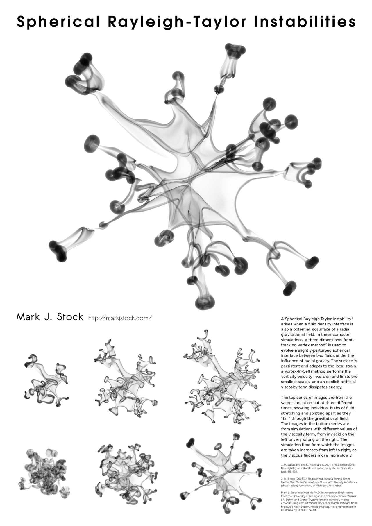
Numerical Rayleigh-Taylor
If you’ve ever dripped food coloring or ink into a glass of water, you’ve probably created a cascade of tiny vortex rings similar to the images above. This is the Rayleigh-Taylor instability, in which the heavier ink/food coloring falls under gravity into the less dense water. What’s shown above is a special case–one that no experiment can recreate. It’s a numerical simulation of a spherical Rayleigh-Taylor instability. Imagine a sphere of a dense fluid “falling” outward under the influence of a radial gravitational field. This is one of the interesting aspects of computational fluid dynamics–it can simulate situations that are impossible to create experimentally. That can be both a strength and a weakness, allowing researchers to probe otherwise unavailable physics or fooling the unwary into thinking they have captured something real. (Image credit: M. Stock)

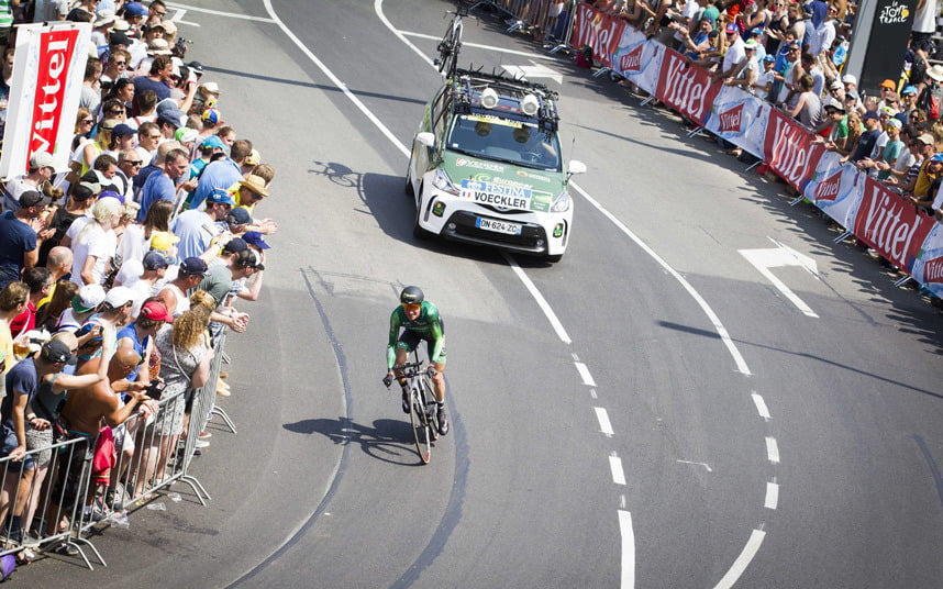
Cars Helping Cyclists

This year’s Tour de France opened with an individual time trial stage in which riders competed solo against the clock. But, according to numerical simulations, some riders may get an unfair aerodynamic advantage in the race if they have a following car. The top image shows the pressure fields around a rider with a car following 5 meters behind versus 10 meters behind. The size of the car means that it displaces air well in advance of its arrival. By following a rider closely, that car’s high pressure region can help fill in a cyclist’s wake, thereby reducing the drag the rider experiences. For a short time trial like the 13.8 km race that kicked off this year’s tour, a rider whose car follows at 5 meter could save 6 seconds over one whose car followed at the regulation 10 meter distance. (As it happens, the stage was decided by a 5 second margin.) Since not all riders get a team follow car, it’s especially important to ensure that those who do aren’t receiving an additional advantage. For more about cycling aerodynamics, check out our previous cycling posts and Tour de France series. (Image credit: TU Eindhoven, EPA/J. Jumelet; via phys.org; submitted by @NathanMechEng)

Jumps in Stratified Flows
One of the factors that complicates geophysical flows is that both the atmosphere and the ocean are stratified fluids with many stacked layers of differing densities. These variations in density can generate instabilities, trap rising or sinking fluids, and transmit waves. The animations above show flow over two ridges with dye visualization (top), velocity (middle), and contours of density (bottom). The upstream influence of the left ridge creates a smooth, focused flow that quickly becomes turbulent after the crest. The jet rebounds as a turbulent hydraulic jump before slowing again upstream of the second ridge. Like the first ridge, the second ridge also generates a hydraulic jump on the lee side. Clearly both stratification and the local topography play a big role in how air moves over and between the ridges. If prevailing winds favor these kinds of flows, it can help generate local microclimates. (Image credit and submission: K. Winters, source videos)


#/media/File:Aileron_roll.gif)