Search results for: “viscous”

  • Featured Video Play Icon

    The Kaye Effect

    The Kaye effect is particular to shear-thinning non-Newtonian fluids – that is, fluids with a viscosity that decreases under deformation. The video above includes high-speed footage of the phenomenon using shampoo. When drizzled, the viscous liquid forms a heap. The incoming jet causes a dimple in the heap, and the local viscosity in this dimple drops due to the shear caused by the incoming jet. Instead of merging with the heap, the jet slips off, creating a streamer that redirects the fluid. This streamer can rise as the dimple deepens, but, in this configuration, it is unstable. Eventually, it will strike the incoming jet and collapse. It’s possible to create a stable version of the Kaye effect by directing the streamer down an incline. (Video credit: S. Lee)

  • Featured Video Play Icon

    When Jets Collide

    When two jets of a viscous liquid collide, they can form a chain-like stream or even a fishbone pattern, depending on the flow rate. This video demonstrates the menagerie of shapes that form not only with changing flow rates but by changing how the jets collide – from a glancing impingement to direct collision. When just touching, the viscous jets generate long threads of fluid that tear off and form tiny satellite droplets. At low flow rates, continuing to bring the jets closer causes them to twist around one another, releasing a series of pinched-off droplets. At higher flow rates, bringing the jets closer to each other creates a thin webbing of fluid between the jets that ultimately becomes a full fishbone pattern when the jets fully collide. The surface-tension-driven Plateau-Rayleigh instability helps drive the pinch-off and break-up into droplets. (Video credit: B. Keshavarz and G. McKinley)

  • Featured Video Play Icon

    Simulating Early Planetary Impacts

    Early in our geological history, Earth was a hellish landscape of molten oceans into which metallic impactors would sometimes collide. Geophysicists have been curious how the impactors behaved after collision: did they maintain their cohesion, or did they break up into a cloud of droplets? Here the UCLA Spinlab simulates this early planetary formation by dropping liquid gallium through a tank of viscous fluid. As the video shows, the impactor’s behavior varies strongly with size. Smaller impactors stick together as a single diapir, but, as the initial size increases, the diapir becomes unstable, eventually breaking down into a cascade of droplets – a metallic rain through an ocean of magma. (Video credit: J. Wacheul et al./UCLA Spinlab; submitted by J. Aurnou)

  • Featured Video Play Icon

    Holiday Fluids: Santa’s Aerodynamics

    Today we have some holiday-themed fluid dynamics: visualization of flow around Santa’s sleigh! This is a flowing soap film visualization at a low speed (author Nick Moore has some other speeds as well). Santa’s sleigh is what aerodynamicists call a bluff body–a shape that is not streamlined or aerodynamic–and sheds a complicated wake of vortices. Like any object moving through a fluid, Santa’s sleigh generates drag forces made up of several components. There is viscous drag, which comes from friction between the sleigh’s surface and the fluid, and form drag (or pressure drag), which comes from the shape of the sleigh. That wake full of complicated vortices significantly increases the sleigh’s pressure drag, requiring Rudolph and the other reindeer to provide more thrust to counter the sleigh’s drag. Speaking thereof, the visualization does not take into account the aerodynamics of the reindeer, who, in addition to providing the sleigh’s thrust, would also affect the flowfield upstream of the sleigh. This post is part of this week’s holiday-themed post series. (Video credit: N. Moore)

  • Reader Question: What is Viscosity?

    Reader Question: What is Viscosity?

    Reader thesnazz asks:

    Is there a difference between surface tension and viscosity, or are they two manifestations of the same process and/or principles? If you know a given fluid’s surface tension, can you predict its viscosity, and vice versa?

    This is a good question! To answer it, let’s think about where surface tension and viscosity come from. Like many concepts in fluid dynamics, these quantities describe for a whole fluid the properties that arise from interactions between molecules.

    To prevent this becoming overly long, I’m going to tackle this over a couple posts. Today, I’ll talk about viscosity.

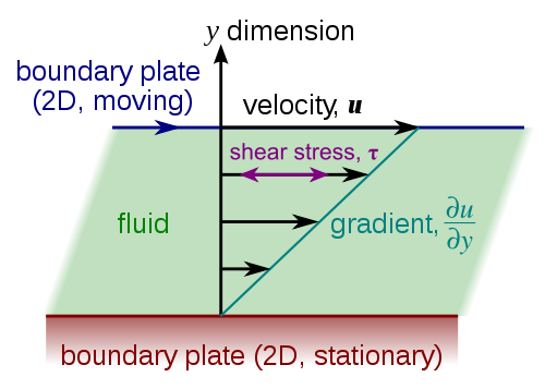
    One way to describe a fluid’s viscosity is as a measure of its resistance to deformation. Another way to think of it is how easily momentum is transmitted from one part of the fluid to another. The diagram above is the classic representation. A layer of fluid is sandwiched between two flat plates. If the top plate moves, friction requires that the fluid particles in contact with the plate get dragged along. This shears the fluid just below that and drags it along, but not quite as much. Those fluid particles do the same to their neighbors and so on down to the stationary second plate, where the fluid is at rest.

    Viscosity is the property that determines how much those neighboring fluid particles move; the more viscous the fluid, the more the neighboring bits of fluid resist getting pulled along. This is a property that’s inherent to a fluid. It comes from how the molecules of the fluid interact with one another, but there are no simple expressions to calculate the viscosity of a liquid or a gas from the individual interactions of its molecules. Instead we experimentally measure viscosity values and use empirical formulas to approximate how viscosity changes with temperature and other effects. (Image credit: Wikimedia)

  • Pitcher Plant Fluid Dynamics

    Pitcher Plant Fluid Dynamics

    Carnivorous pitcher plants owe much of their efficacy to the viscoelasticity of their digestive fluid. A viscoelastic fluid’s resistance to deformation has two components: the usual viscous component that resists shearing and an elastic component, often derived from the presence of polymers, that resists stretching – kind of like a liquid rubber band. It’s the latter effect that’s important when it comes to the pitcher plant trapping insects. When a fly or ant falls into the liquid within the plant, it will flail and try to swim, thereby straining the fluid. In part © of the image above, you can see how long fluid filaments stretch as the fly moves; this is because the digestive fluid’s extensional viscosity, the elastic component, is 10,000 times larger than its shear viscosity, the usual viscous component, for motions like the fly’s. This viscoelastic fluid is so effective at trapping insects that, as seen in part (b) above, it has to be diluted by more than 95% before insects can escape it! (Image credit: L. Gaume and Y. Forterre)

  • Bubbles Through Constrictions

    Bubbles Through Constrictions

    Surface tension usually constrains bubbles to the smallest area for a given volume – a sphere – but sometimes other forces generate more complicated geometries. The images above show bubbles flowing through microfluidic channels filled with a highly viscous carrier fluid. The bubble size and packing affects the shapes they assume, but so does the geometry of the channel. The narrow constrictions accelerate the flow, elongating the bubbles, whereas the wider channel regions slow the carrier fluid and squish the bubbles together. (Image credit: M. Sauzade and T. Cubaud (Stony Brook University))

  • Featured Video Play Icon

    Holey Splashes

    A liquid’s surface tension can have a big effect on its splashes. In this video, a 5-mm droplet hits a surface covered in a thin layer of a liquid with lower viscosity and surface tension. The result is a dramatic effect on the spreading splash. As the initial curtain grows and expands, the lower surface tension of the impacted fluid thins the splash curtain. Fluid flows away from these areas due to the Marangoni effect, causing holes to grow. The sheet breaks up into a network of liquid filaments and ejected droplets before gravity can even bring it all to rest. For more, see this previous post and review paper. (Video credit: S. Thoroddsen et al.)

  • Featured Video Play Icon

    The Reynolds Number Illustrated

    The dimensionless Reynolds number is a key concept in fluid dynamics, allowing scientists to distinguish regimes of flow between differing geometries and even different fluids. This video gives a great primer on the subject by examining the physics of swimming for a sperm versus a sperm whale. The Reynolds number is essentially a ratio between inertial forces (driven by velocity and size) and viscous forces, and its value can indicate how important different effects are. Sperm and other microbes live at very small Reynolds numbers, meaning that viscosity dominates as the force they must overcome to move. For more on the low Reynolds number world, check out how brine shrimp swim and what happens if a microbe tries to flap its tail. (Hint: it goes nowhere, and this is why.) (Video credit: A. Bhatia/TED Ed; via Jennifer Ouellette)

  • Other Ig Nobel Fluids

    Other Ig Nobel Fluids

    To round out our series on fluid dynamics in the Ig Nobel Prizes (which are not the same thing as the actual Nobel Prizes), here are some of the other winners. Last year Mayer and Krechetnikov won for a study on coffee sloshing when people walk. We’ve mentioned the pitch-drop experiment measuring the viscosity of an extremely viscous fluid a couple times; Mainstone and Parnell won a 2005 Ig Nobel for that (on-going) work. Another 2005 prize went to Meyer-Rochow and Gal for calculating the pressures involved in penguin defecation. (Yes, seriously.) A avian-related award was also handed out to B. Vonnegut for estimating tornado wind speeds by their ability to strip a chicken of its feathers. And, finally, for those looking to interest undergraduate lab students in mathematics and fluid dynamics, I suggest following the lead of 2002 winner A. Leike who demonstrates laws of exponential decay with beer head. (Photo credit: S. Depolo)