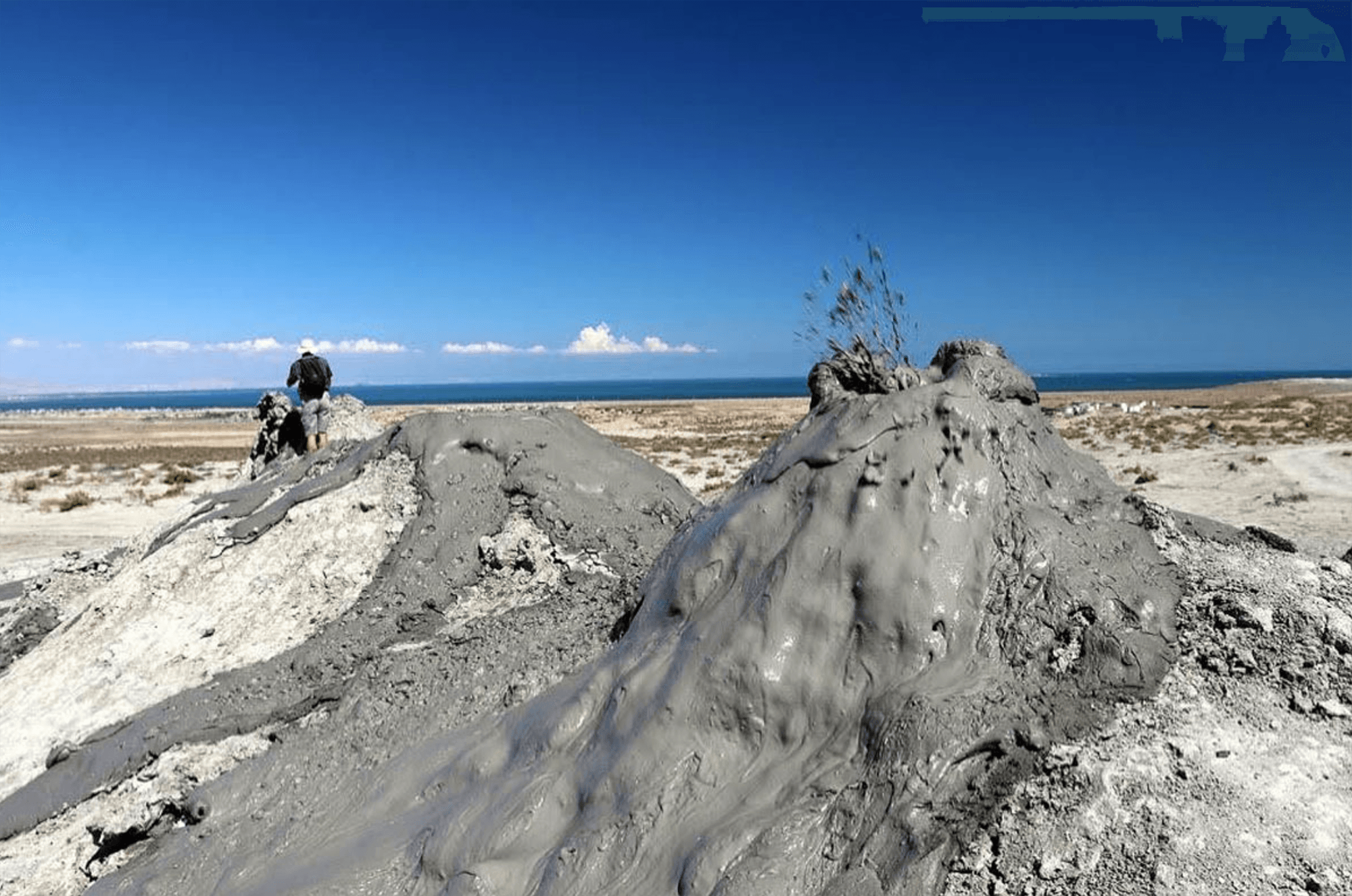
Mars features mounds that resemble our terrestrial mud volcanoes, suggesting that a similar form of mudflow occurs on Mars. But Mars’ thin atmosphere and frigid temperatures mean that water — a prime ingredient of any mud — is almost always in either solid or gaseous form on the planet. So researchers explored whether salty muds could flow under Martian conditions. They tested a variety of salts, at different concentrations, in a low-pressure chamber calibrated to Mars-like temperatures and pressures. The salts lowered water’s freezing point, allowing the muds to remain fluid. Even a relatively small amount of sodium chloride — 2.5% by weight — allowed muds to flow far. The team also found that the salt content affected the shape the flowing mud took, with flows ranging from narrow, ropey patterns to broad, even sheets. (Image credit: P. Brož/Wikimedia Commons; research credit: O. Krýza et al.; via Eos)
Tag: planetary science

Climate Change and the Equatorial Cold Tongue
A cold region of Pacific waters stretches westward along the equator from the coast of Ecuador. Known as the equatorial cold tongue, this region exists because trade winds push surface waters away from the equator and allow colder, deeper waters to surface. Previous climate models have predicted warming for this region, but instead we’ve observed cooling — or at least a resistance to warming. Now researchers using decades of data and new simulations report that the observed cooling trend is, in fact, a result of human-caused climate changes. Like the cold tongue itself, this new cooling comes from wind patterns that change ocean mixing.
As pleasant as a cooling streak sounds, this trend has unfortunate consequences elsewhere. Scientists have found that this cooling has a direct effect on drought in East Africa and southwestern North America. (Image credit: J. Shoer; via APS News)
Fediverse Reactions
-

Inside an Alien Atmosphere
Studying the physics of planetary atmospheres is challenging, not least because we only have a handful of examples to work from in our own solar system. So it’s exciting that researchers have unveiled our first look at the 3D structure of an exoplanet‘s atmosphere.
Using ground-based observations, researchers studied WASP-121b, also known as Tylos, an ultra-hot Jupiter that circles its star in only 30 Earth hours. One face of the planet always faces its star while the other faces into space. The team found that the exoplanet has a flow deep in the atmosphere that carries iron from the hot daytime side to the colder night side. Higher up, the atmosphere boasts a super-fast jet-stream that doubles in speed (from an estimated 13 kilometers per second to 26 kilometers per second) as it crosses from the morning terminator to the evening. As one researcher observed, the planet’s everyday winds make Earth’s worst hurricanes look tame. (Image credit: ESO/M. Kornmesser; research credit: J. Seidel et al.; via Gizmodo)
Fediverse Reactions
-

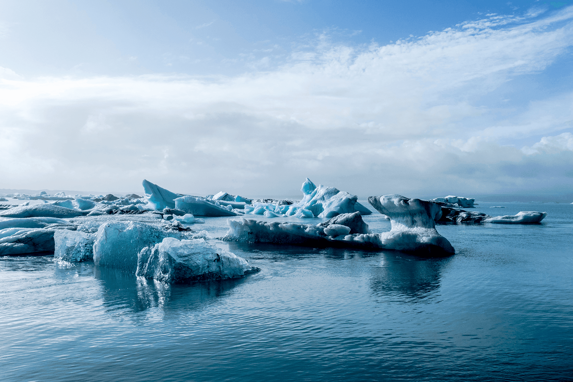
Growing Ice
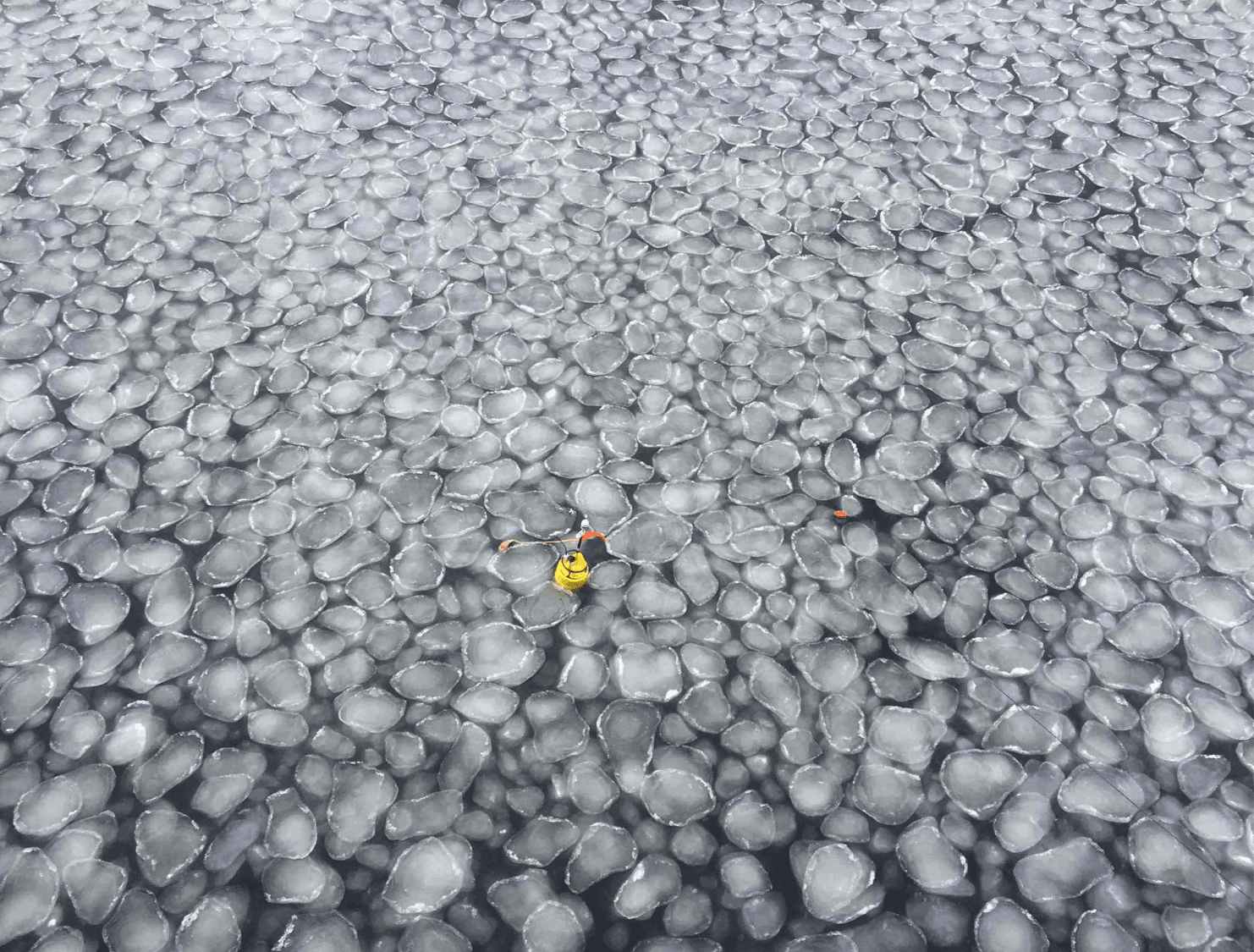
While much attention is given to the summer loss of sea ice, the birth of new ice in the fall is also critical. Ice loss in the summer leaves oceans warmer and waves larger since wind can blow across longer open stretches. Those warmer waters and more dynamic waves affect how ice forms once autumn sets in. Higher waves mean that ice tends to form in “pancakes” like those seen here. Pancake ice is small — typically under 1 meter wide — and can only be observed from nearby, since they’re smaller than typical satellite resolution. Only once there’s enough pancake ice to dampen the waves will the pieces begin to cement together to form larger pieces that will form the basis of the year’s new ice. (Image credit: M. Smith; see also Eos)
Fediverse Reactions
-

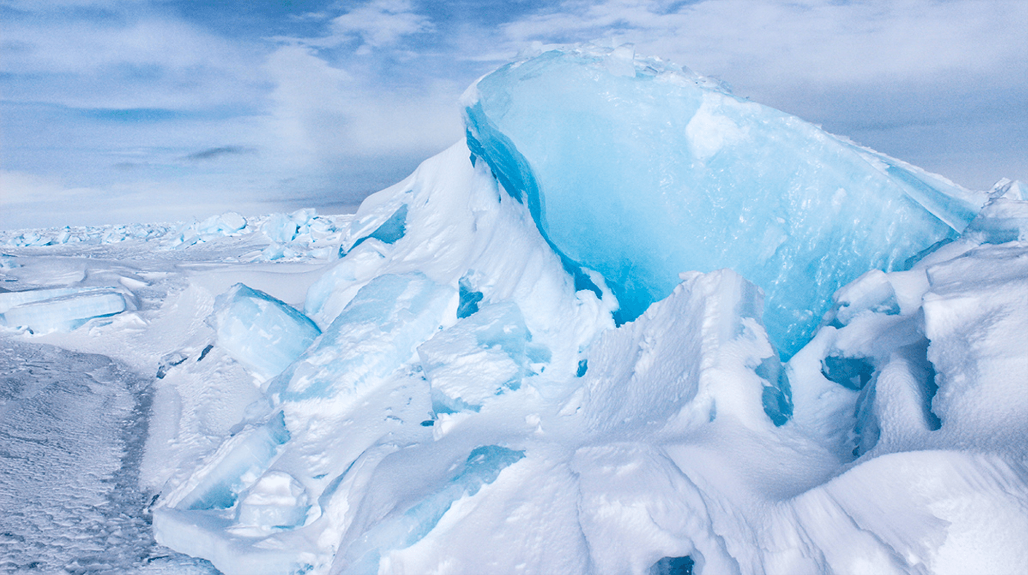
Disappearing Sea Ice Ridges
As blocks of sea ice shift and float, they can press together, forming ridges spaced every few hundred meters or so. A new study uses aerial observations from recent decades to show that these sea ridges are getting smaller in both size and number, a smoothing of Arctic topography that has many consequences.
The team showed that the overall changes in the sea ridges correspond to a loss of older sea ice. The current smoother sea ice presents less drag to winds and currents, which might suggest that the ice is slower-moving, but instead the opposite seems true. Scientists are not sure why the ice is moving faster, though faster ocean currents may play a role.
Another consequence of smoother sea ice is wider, shallower melt ponds each summer. These wider ponds increase the amount of sunlight the ice absorbs, hastening melting even further. (Image credit: USGS; research credit: T. Krumpen et al.; via Eos)

An Exoplanet’s Supersonic Jet Stream
WASP-127b is a hot Jupiter-type exoplanet located about 520 light-years from us. A new study of the planet’s atmosphere reveals a supersonic jet stream whipping around its equatorial region at 9 kilometers per second. For comparison, our Solar System’s fastest winds, on Neptune, are a comparatively paltry 0.5 kilometers per second. The team estimates the speed of sound — which depends on temperature and the atmosphere’s chemical make-up — on WASP-127b as about 3 kilometers per second, far below the measured wind speed. The planet’s poles, in contrast, are much colder and have far lower wind speeds.
Of course, these measurements can only give us a snapshot of what the exoplanet’s atmosphere is like; we don’t have altitude data, for example, to see how the wind speed varies with height. Nevertheless, it shows that exoplanets beyond our planetary system can have some unimaginably wild weather. (Video and image credit: ESO/L. Calçada; research credit: L. Nortmann et al.; via Gizmodo)
Fediverse Reactions
-

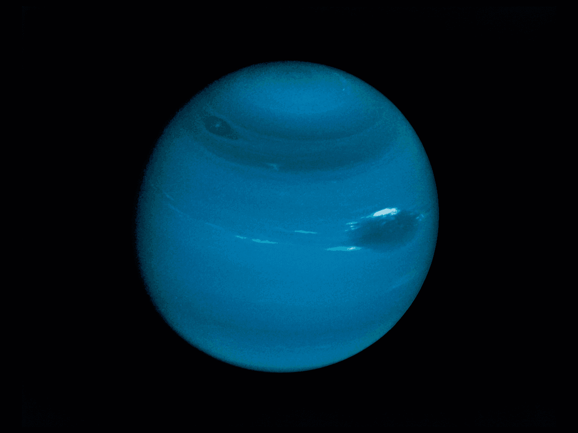
Why Icy Giants Have Strange Magnetic Fields
When Voyager 2 visited Uranus and Neptune, scientists were puzzled by the icy giants’ disorderly magnetic fields. Contrary to expectations, neither planet had a well-defined north and south magnetic pole, indicating that the planets’ thick, icy interiors must not convect the way Earth’s mantle does. Years later, other researchers suggested that the icy giants’ magnetic fields could come from a single thin, convecting layer in the planet, but how that would look remained unclear. Now a scientist thinks he has an answer.
When simulating a mixture of water, methane, and ammonia under icy giant temperature and pressure conditions, he saw the chemicals split themselves into two layers — a water-hydrogen mix capable of convection and a hydrocarbon-rich, stagnant lower layer. Such phase separation, he argues, matches both the icy giants’ gravitational fields and their odd magnetic fields. To test whether the model holds up, we’ll need another spacecraft — one equipped with a Doppler imager — to visit Uranus and/or Neptune to measure the predicted layers firsthand. (Image credit: NASA; research credit: B. Militzer; via Physics World)
Fediverse Reactions
-

Tracking Coastal Sediment Loss
Shorelines rely on an influx of sediment to counter what’s lost to erosion by waves and currents. But tracking that sediment flux is challenging in coastal regions where salt, waves, and storms batter delicate instruments. Instead, researchers have turned to remote sensing through high-resolution satellites like Landsat to monitor these areas. Researchers built an algorithm to analyze coastal imagery, validated with local sediment measurements; once built, they deployed it in a free tool that lets anyone build a 40-year timeline of a coastal area’s sediment history.
Looking at thousands of sites around the world, the team found coastal sediment is on the decline, especially along sandy and muddy coastlines. Where has the sediment gone? It’s likely that human-built infrastructure — both on coasts and upstream along rivers — is disrupting the natural flow of sediments that would replenish these regions. (Image credit: NASA; research credit: W. Teng et al.; via Eos)
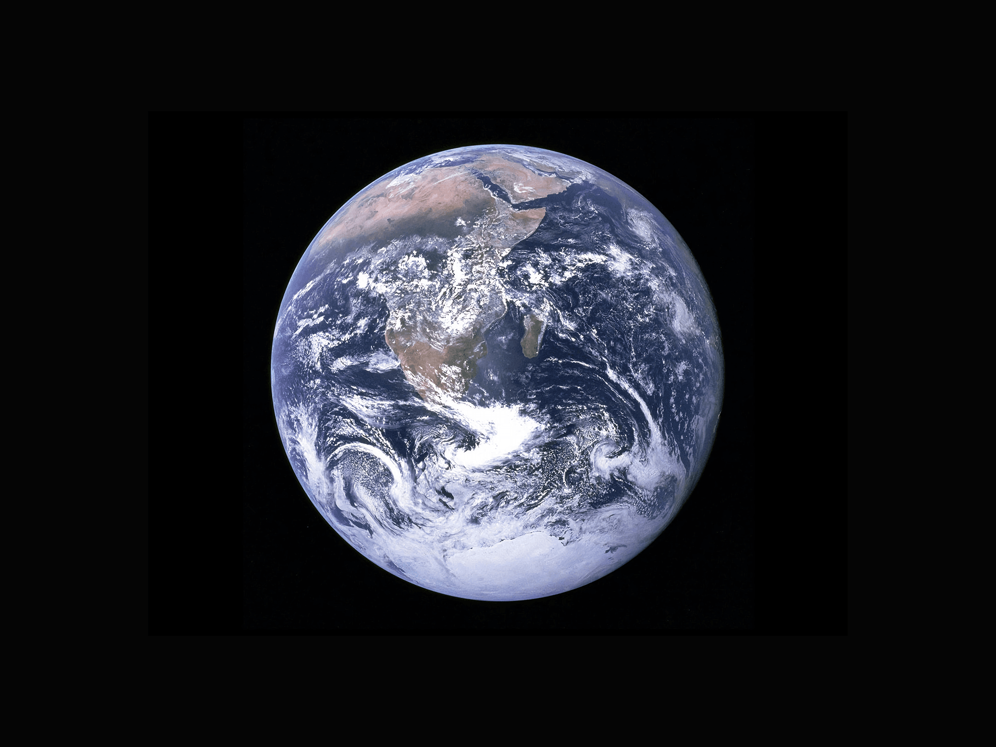
A New Mantle Viscosity Shift
The rough picture of Earth’s interior — a crust, mantle, and core — is well-known, but the details of its inner structure are more difficult to pin down. A recent study analyzed seismic wave data with a machine learning algorithm to identify regions of the mantle where waves slowed down. These shifts in seismic wave speed occur in areas where the mantle’s viscosity changes; a higher viscosity makes waves travel slower.
The team found seismic wave speed shifts at depths of 400 and 650 kilometers, corresponding to known viscosity changes. But they found shifts at 1050 and 1500 kilometers, as well — the first time anyone has shown a global viscosity shift at those depths. Their analysis suggests a higher viscosity in this mid-mantle transition zone, which could affect how tectonic plates, which rely on these slow mantle flows, move. (Image credit: NASA; research credit: K. O’Farrell and Y. Wang; via Eos)

Tracking Ice Floes
To understand why some sea ice melts and other sea ice survives, researchers tracked millions of floes over decades. This herculean undertaking combined satellite data, weather reports, and buoy data into a database covering nearly 20 years of data. With all of that information, the team could track the changes to specific pieces of ice rather than lumping data into overall averages.
They found that an ice floe’s fate depended strongly on the route it took: ice that slipped from its starting region into warmer, more southern regions was likely to melt. They also saw region-specific effects, like that thick sea ice was more likely to melt in the East Siberian Sea’s summer, possibly due to warmer currents. The comprehensive, fine-grained analyses possible with this ice-tracking technique offer a chance to understand why some Arctic regions are more vulnerable to warming than others. (Image credit: D. Cantelli; research credit: P. Taylor et al.; via Eos)


.JPG)