
Smoke visualization in a wind tunnel shows the vortices wrapping around and trailing behind a delta wing. As with more commonly seen rectangular or swept wings, the vortices that form around delta wings affect lift, drag, and control of an aircraft. They can also be hazardous to aircraft nearby. Note that, although delta wings are often seen on supersonic aircraft, this visualization only applies at subsonic speeds. The flow field changes drastically above the speed of sound.
Month: September 2011
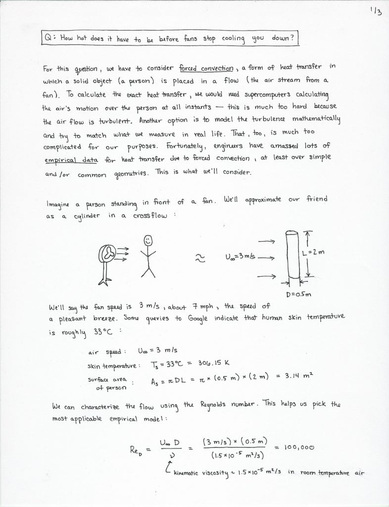
Reader Question: How Hot Can It Be Before a Fan Stops Cooling You?
lazenby asks:
This isn’t strictly a dynamics question, but I was wondering how hot a stream of fluid has to be before it can no longer lower the average temperature of a body placed in its flow. As an example, how hot a day does it have to be before fans stop cooling you down? What’s the relation and the math to reach for here?
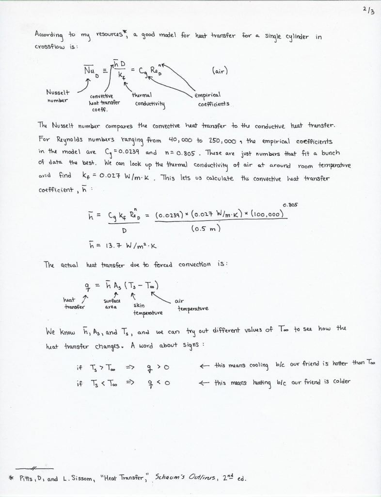
Wonder no further! You seek the subject of heat transfer–specifically forced convection. Here’s a brief look at how to calculate the cooling due to a fan. Click to enlarge each page.


Airfoil Boundary Layer
This video shows the turbulent boundary layer on a NACA 0010 airfoil at high angle of attack (15 degrees). Notice how substantial the variations are in the boundary layer over time. At one instant the boundary layer is thick and smoke-filled and in another we see freestream fluid (non-smoke) reaching nearly to the surface. This variability, known as intermittency, is characteristic of turbulent flows, and is part of what makes them difficult to model.

Microgravity Combustion
This collage of three combustion images reveals the beautiful symmetry of flames in microgravity. In the absence of gravity, flames are spherical, and, in the confines of a spacecraft, any combustion is extremely dangerous. Thus, most microgravity combustion experiments occur in drop towers. From NASA:
Each image is of flame spread over cellulose paper in a spacecraft ventilation flow in microgravity. The different colors represent different chemical reactions within the flame. The blue areas are caused by chemiluminescence (light produced by a chemical reaction.) The white, yellow and orange regions are due to glowing soot within the flame zone. #
Surface Tension Demo
This simple demonstration shows the power of surface tension, especially at small lengthscales. Another way to break the surface tension holding the water in the sieve would be to spray the top of the jar with soapy water. The soap acts as surfactant, decreasing the surface tension such that the water is unable to counteract the force of gravity.

Impinging Without Coalescing
Three impinging jets of silicone oil rebound without coalescence due to thin-film lubrication between the jets. The motion of the oil replenishes the thin layer of air separating the streams. The same phenomenon keeps droplets from coalescing as well. (Photo credit: BIF Lab, Department of Engineering Science and Mechanics, Virginia Tech) #
Blast Waves
[original media no longer available]
Watch closely in this high-speed video of a bomb exploding and you will see the spherical blast wave moving outward as a visual distortion. The increase in temperature caused by the leading shockwave changes the index of refraction of the air, bending the light and distorting our view of the background. The mechanism is similar to schlieren photography, which has been used for more than a century to capture images of compressible flows.
2D Convection
This simulation shows 2D Rayleigh-Benard convection in which a fluid of uniform initial temperature is heated from below and cooled from above. This is roughly analogous to the situation of placing a pot of water on a hot stovetop. (In the case of the water on the stove, the upper boundary is the water-air interface, while, in the simulation, the upper boundary is modeled as a no-slip (i.e. solid) interface.) The simulation shows contours of temperature (black = cool, white = hot). In general, the hot fluid rises and the cold fluid sinks due to differences in density, but, as the simulation shows, the actual mixing that occurs is far more complex than that simple axiom indicates.
Reader Question: Faucet Physics
jessecaps-blog-deactivated20170 asks:
With respect to the laminar/turbulent flow in the faucet, at the end he explains that the diameter is smaller inside the valve compared to the nozzle and therefore the velocity is greater and turbulence is achieved there before it leaves the nozzle. But turbulence is characterized by the Reynolds number not the velocity, so a larger velocity with a smaller diameter will yield the same Reynolds number, why would we expect turbulence in the nozzle before the stream?
ETA: As pointed out in the comments, I made a very silly mistake when calculating the Reynolds number last night. While most of what I say below is still true in general, it’s not in the case in the faucet, and so I’ve edited the entry to reflect that.
Great question! A quick control volume analysis of an incompressible fluid shows that, while the flow speed is higher through the faucet’s valve, the Reynolds number (based on diameter) at the valve is the same as higher than the Reynolds number at the nozzle by a factor of (nozzle diameter)/(valve diameter). Thus transition can occur at the valve before the nozzle. A word of caution, though: although we often use Reynolds number as a method of characterizing when a flow becomes turbulent, it is not a hard and fast rule.
As undergraduates we learn that pipe flow transitions to turbulence at a Reynolds number of 2,300 based on the pipe’s diameter. However, under the right laboratory conditions, it’s possible to maintain laminar flow in a pipe to a Reynolds number an order of magnitude larger. (#) It all depends on the initial conditions of the flow and the influence of factors like surface roughness. What this means in the case of the faucet is that the same Reynolds number (based on diameter) may not correctly indicate whether the flow is laminar or turbulent at a given point.
Now, while it may be possible that the contraction at the valve introduces some small turbulence that decays prior to the flow’s exit from the nozzle, that does not seem overly likely to me. Even though, by Reynolds number, transition can occur at the valve before the nozzle, I suspect most of the sound we hear comes from the increased flow rate caused by turning the faucet. It may also be that the sound is associated with the onset of turbulence at the valve but the turbulence is still slight enough that we do not notice it by eye in the external flow.
Laminar and Turbulent Flows from a Faucet
Here laminar and turbulent flows, basic concepts in fluid mechanics, are demonstrated in the kitchen sink! While laminar flow is often desirable for decreasing drag due to friction, most practical flows are turbulent. The hissing the video author associates with the onset of turbulence is not a coincidence either. The chaotic motion of turbulent flows can produce aerodynamic noise like the roar produced by airplane propellers or the hum of electrical lines in the wind.


