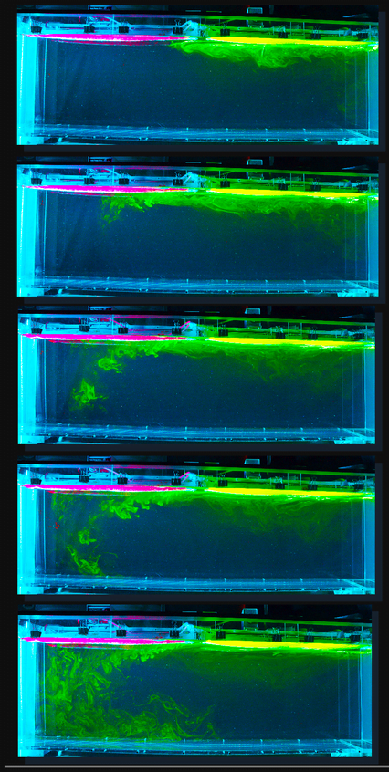
Earth’s oceans are a complex and dynamic environment, but fortunately, we can simulate some of their physics on a smaller scale in the laboratory. The time series of images above show how fresh and salty waters mix. On the right side of the image is fresh water with its top layer dyed green. On the left is salty water dyed pink. Initially, the fresh water spreads horizontally toward the salty region in a smooth and laminar fashion. As the fresh water picks up salt, it gets denser and starts sinking, ultimately forming a turbulent plume that will push all the way back across the tank. For more images, check out the full poster. (Image credit: P. Passaggia et al.)
Tag: turbulence

Inside a Cello
At first glance, Adrian Borda’s photograph seems to show an old room. In reality, this is the interior of a cello with light shining through the f-holes. Dust particles in the air trace out pathlines that reveal the turbulent movements of air inside the instrument. Both the camera’s perspective and the visible flow try to trick our minds into seeing something larger than reality. It’s a reminder that the patterns and forms of fluid flow repeat across an enormous range of scales, from millimeters to light-years. (Image credit: A. Borda; via Joseph S./CU Boulder Flow Viz)

Soap Film Turbulence
The brilliant colors of a soap film reveal the fluid’s thickness, thanks to a process known as thin film interference. The twisting flow of the film depends on many influences: gravity pulls down on the liquid and tends to make it drain away; evaporation steals fluid from the film; local air currents can push or pull the film; and the variation in the concentration of molecules – specifically the surfactants that stabilize the film – will change the local surface tension, causing flow via the Marangoni effect. Together these and other effects create the dancing turbulence captured above. (Video credit: A. Filipowicz)

Where Does the Sun End?
How do you define the edge of our sun? There’s a distinct surface to it, but our star is also surrounded by the corona, an even hotter region of plasma twisted by magnetic fields. The corona is sort of like the sun’s atmosphere. Farther out in the solar system, we receive a constant barrage of charged particles, known as the solar wind, that streams out from the sun. So where does the corona end and the solar wind begin?
Scientists have been studying the flow structure of the solar wind in search of an answer to this question, and they’ve found that there’s a clear transition point about 32 million kilometers from the sun. At this distance, the sun’s magnetic field weakens to the point where it no longer exerts the same hold on the solar particles and they begin to move turbulently, behaving more like a gas than a plasma. With special measurements and image processing, scientists were able to actually see this flow change in the solar wind! (Video/image credit: NASA; research credit: C. DeForest et al.; via FlowViz)


Turbulence in the Solar Wind
One of the key features of turbulent flows is that they contain many different length scales. Look at the plume from an erupting volcano, and you’ll see eddies that are hundreds of meters across as well as tiny ones on the order of millimeters. This enormous difference in scale is one of the major challenges in simulating turbulent flows. Since energy enters at the large scale and is passed to smaller and smaller scales before being dissipated at the tiniest scales of the flow, properly simulating a turbulent flow requires resolving all of these length scales. This is especially challenging for applications like the solar wind – the stream of charged particles that flows from the sun and gets diverted around the Earth by our magnetic field. The image above shows some of the turbulence in our solar wind. The structures seen in the flow range from the size of the Earth all the way to the scale of electrons! (Image credit: B. Loring, Berkeley Lab)

Flamethrowing
Humans have long been fascinated by staring into flames, and the Slow Mo Guys carry on the grand tradition here with 4K, high-speed video of a flamethrower. Like firebreathers, a flamethrower’s fire is the result of a spray of tiny, volatile droplets of fuel. Once ignited, the spray becomes a turbulent jet of flames. Turbulent flows are known for having both large and small-scale structure, and there’s some really great close-ups showing this around the 2:00 mark. Also watch the edges of the flame, where the nearby air has gotten hot enough to shimmer. You can see how the trees in the background ripple and blur as the fire heats up the air and changes its density and refractive index. (Video credit: The Slow Mo Guys)

Visualizing Smell
Every day we’re surrounded by an invisible world of smells. Like the fluorescein dye in the animation above, these odors drift and swirl in the background flow. What you may not have stopped to consider when you smell the roses, though, is how the very act of sniffing changes the scent. When you inhale, filaments of the odor are drawn into your nose, and, likewise, when you exhale, your breathe mixes with the scent and sends it swirling outward in turbulent eddies. To see more about the science of scent, check out PBS News Hour’s full video below. (Video credit: PBS News Hour; GIF via skunkbear)

Bumblebees in Turbulence

Bumblebees are small all-weather foragers, capable of flying despite tough conditions. Given the trouble that micro air vehicles have when flying in gusty winds, bumblebees can help engineers to understand how nature successfully deals with turbulence. Under smooth laminar conditions like those shown in the animation above, bumblebees stay aloft by beating their wings forward and backward in a figure-8-like motion. On both the forward downstroke and the backward upstroke, you’ll notice a blue bulge near the front of the bee’s wing. This is a leading-edge vortex, which provides much of the bee’s lift.
Researchers were curious how adding turbulence would affect their virtual bee’s flight. The still image above shows the bee in moderate freestream turbulence (shown in cyan). Surprisingly, this outside turbulence has very little effect on the flow generated by the bee, shown in pink. In fact, the researchers found that the bees could fly through turbulence without a significant increase in power. Too much turbulence does make it hard for the bee to control its flight, though. The bee’s shape makes it prone to rolling, and the researchers estimated, based on a bee’s 20 ms reaction time, that bumblebees can probably only correct that roll and maintain controlled flight at turbulence intensities less than 63% of the mean wind speed. (Image credits: T. Engels et al., source; via Physics Focus)

Eulerian vs. Lagrangian

When I first studied fluid dynamics, one of the concepts I struggled with was that of Eulerian and Lagrangian reference frames. Essentially, these are just two different perspectives you can view the fluid from. Physics is the same in both, but mathematically, you approach them differently. In the Eulerian perspective one sits at a location and watches the flow pass, like an observer watching a river go by. It’s demonstrated in the top animation, where turbulent flow sweeps past in a pipe. This is the usual perspective experimentally – you put an instrument at a certain point in the flow and you gather information as the fluid streams past in time.


In the Lagrangian perspective, on the other hand, one follows a particular bit of fluid around and observes its changes over time. This means that one has to follow along at the mean speed of the flow in order to keep up with the fluid parcel one is observing. It would be like running alongside a river so that you can always be watching the same water as it flows downstream. The Lagrangian view of the same turbulent pipe flow is shown in the bottom animation. Notice how moving alongside the pipe makes it easier to see how the turbulence morphs as it goes along. Experimentally, this can be harder to achieve (at least in a flow with non-zero mean speed), but it’s a useful method of studying unsteadiness. (Image credit: J. Kühnen et al., source)

Dyeing the River
Every year Chicago dyes part of its river green to celebrate St. Patrick’s Day. This timelapse video gives a great view of the 2016 dyeing. If you watch closely, you’ll see that what’s being put in the river isn’t originally green. It’s actually an orange powder being distributed through flour sifters by the men on the boat. The exact formula is secret, but the dye is considered environmentally safe. To mix up the dye, a chase boat follows the dye boat, using its motor and wake structure to help add some turbulence to the river. It takes several passes to get the water uniformly green, but it requires a remarkably small amount of dye to do so, only about a paint can’s worth. So enjoy a little fluid dynamics today with your festivities! (Or, if you prefer to celebrate a different sort of fluid dynamics today, allow me to offer you the physics of Guinness.) (Video credit: Chris B Photo)


