Tag: planetary science

An Exoplanet’s Supersonic Jet Stream
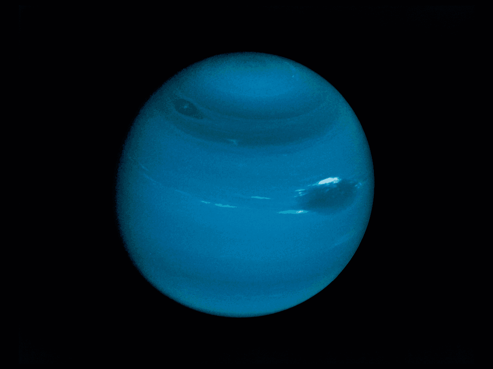
WASP-127b is a hot Jupiter-type exoplanet located about 520 light-years from us. A new study of the planet’s atmosphere reveals a supersonic jet stream whipping around its equatorial region at 9 kilometers per second. For comparison, our Solar System’s fastest winds, on Neptune, are a comparatively paltry 0.5 kilometers per second. The team estimates the speed of sound — which depends on temperature and the atmosphere’s chemical make-up — on WASP-127b as about 3 kilometers per second, far below the measured wind speed. The planet’s poles, in contrast, are much colder and have far lower wind speeds.
Of course, these measurements can only give us a snapshot of what the exoplanet’s atmosphere is like; we don’t have altitude data, for example, to see how the wind speed varies with height. Nevertheless, it shows that exoplanets beyond our planetary system can have some unimaginably wild weather. (Video and image credit: ESO/L. Calçada; research credit: L. Nortmann et al.; via Gizmodo)
Fediverse Reactions
February 11, 2025
Why Icy Giants Have Strange Magnetic Fields
When Voyager 2 visited Uranus and Neptune, scientists were puzzled by the icy giants’ disorderly magnetic fields. Contrary to expectations, neither planet had a well-defined north and south magnetic pole, indicating that the planets’ thick, icy interiors must not convect the way Earth’s mantle does. Years later, other researchers suggested that the icy giants’ magnetic fields could come from a single thin, convecting layer in the planet, but how that would look remained unclear. Now a scientist thinks he has an answer.
When simulating a mixture of water, methane, and ammonia under icy giant temperature and pressure conditions, he saw the chemicals split themselves into two layers — a water-hydrogen mix capable of convection and a hydrocarbon-rich, stagnant lower layer. Such phase separation, he argues, matches both the icy giants’ gravitational fields and their odd magnetic fields. To test whether the model holds up, we’ll need another spacecraft — one equipped with a Doppler imager — to visit Uranus and/or Neptune to measure the predicted layers firsthand. (Image credit: NASA; research credit: B. Militzer; via Physics World)
Fediverse Reactions
January 16, 2025
Tracking Coastal Sediment Loss
Shorelines rely on an influx of sediment to counter what’s lost to erosion by waves and currents. But tracking that sediment flux is challenging in coastal regions where salt, waves, and storms batter delicate instruments. Instead, researchers have turned to remote sensing through high-resolution satellites like Landsat to monitor these areas. Researchers built an algorithm to analyze coastal imagery, validated with local sediment measurements; once built, they deployed it in a free tool that lets anyone build a 40-year timeline of a coastal area’s sediment history.
Looking at thousands of sites around the world, the team found coastal sediment is on the decline, especially along sandy and muddy coastlines. Where has the sediment gone? It’s likely that human-built infrastructure — both on coasts and upstream along rivers — is disrupting the natural flow of sediments that would replenish these regions. (Image credit: NASA; research credit: W. Teng et al.; via Eos)
January 14, 2025
A New Mantle Viscosity Shift
The rough picture of Earth’s interior — a crust, mantle, and core — is well-known, but the details of its inner structure are more difficult to pin down. A recent study analyzed seismic wave data with a machine learning algorithm to identify regions of the mantle where waves slowed down. These shifts in seismic wave speed occur in areas where the mantle’s viscosity changes; a higher viscosity makes waves travel slower.
The team found seismic wave speed shifts at depths of 400 and 650 kilometers, corresponding to known viscosity changes. But they found shifts at 1050 and 1500 kilometers, as well — the first time anyone has shown a global viscosity shift at those depths. Their analysis suggests a higher viscosity in this mid-mantle transition zone, which could affect how tectonic plates, which rely on these slow mantle flows, move. (Image credit: NASA; research credit: K. O’Farrell and Y. Wang; via Eos)
January 7, 2025
Tracking Ice Floes
To understand why some sea ice melts and other sea ice survives, researchers tracked millions of floes over decades. This herculean undertaking combined satellite data, weather reports, and buoy data into a database covering nearly 20 years of data. With all of that information, the team could track the changes to specific pieces of ice rather than lumping data into overall averages.
They found that an ice floe’s fate depended strongly on the route it took: ice that slipped from its starting region into warmer, more southern regions was likely to melt. They also saw region-specific effects, like that thick sea ice was more likely to melt in the East Siberian Sea’s summer, possibly due to warmer currents. The comprehensive, fine-grained analyses possible with this ice-tracking technique offer a chance to understand why some Arctic regions are more vulnerable to warming than others. (Image credit: D. Cantelli; research credit: P. Taylor et al.; via Eos)
December 31, 2024
Beneath a River of Red
A glowing arch of red, pink, and white anchors this stunning composite astrophotograph. This is a STEVE (Strong Thermal Emission Velocity Enhancement) caused by a river of fast-moving ions high in the atmosphere. Above the STEVE’s glow, the skies are red; that’s due either to the STEVE or to the heat-related glow of a Stable Auroral Red (SAR) arc. Find even more beautiful astrophotography at the artist’s website and Instagram. (Image credit: L. Leroux-Géré; via APOD)
Fediverse Reactions
December 20, 2024
How Magnetic Fields Shape Core Flows
The Earth’s inner core is a hot, solid iron-rich alloy surrounded by a cooler, liquid outer core. The convection and rotation in this outer core creates our magnetic fields, but those magnetic fields can, in turn, affect the liquid metal flowing inside the Earth. Most of our models for these planetary flows are simplified — dropping this feedback where the flow-induced magnetic field affects the flow.
The simplification used, the Taylor-Proudman theorem, assumes that in a rotating flow, the flow won’t cross certain boundaries. (To see this in action, check out this Taylor column video.) The trouble is, our measurements of the Earth’s actual interior flows don’t obey the theorem. Instead, they show flows crossing that imaginary boundary.
To explore this problem, researchers built a “Little Earth Experiment” that placed a rotating tank (representing the Earth’s inner and outer core) filled with a transparent, magnetically-active fluid inside a giant magnetic. This setup allowed researchers to demonstrate that, in planetary-like flows, the magnetic field can create flow across the Taylor-Proudman boundary. (Image credit: C. Finley et al.; research credit: A. Pothérat et al.; via APS Physics)
November 21, 2024
The Great Red Spot’s Cycle
First spotted by humanity in 1664, Jupiter‘s Great Red Spot is a seemingly endless storm. Strictly speaking, there is debate as to whether observations prior to 1831 were of the same storm, but there’s no denying that the storm has raged unabated since regular observations began in the first half of the nineteenth century. Despite its longevity, the Great Red Spot is not unchanging. Overall, its major axis is shrinking, making the storm more circular over time. The storm also has a 90-day cycle in which its size, shape, and brightness vary, as seen below. Researchers note that the changes are relatively subtle — at least to the eye — but now that they’ve been identified, it may be possible to use amateur astronomers’ data to track these variations more closely. (Image credits: GRS – K. Gill/NASA, snapshots – A. Simon et al.; research credit: A. Simon et al.; via Gizmodo)
Over a 90 day cycle, Jupiter’s Great Red Spot oscillates in size, shape, and other characteristics.
October 29, 2024
Slushy Snow Affects Antarctic Ice Melt
More than a tenth of Antarctica’s ice projects out over the sea; this ice shelf preserves glacial ice that would otherwise fall into the Southern Ocean and raise global sea levels. But austral summers eat away at the ice, leaving meltwater collected in ponds (visible above in bright blue) and in harder-to-spot slush. Researchers taught a machine-learning algorithm to identify slush and ponds in satellite images, then used the algorithm to analyze nine years’ worth of imagery.
The group found that slush makes up about 57% of the overall meltwater. It is also darker than pure snow, absorbing more sunlight and leading to more melting. Many climate models currently neglect slush, and the authors warn that, without it, models will underestimate how much the ice is melting and predict that the ice is more stable than it truly is. (Image credit: Copernicus Sentinel/R. Dell; research credit: R. Dell et al.; via Physics Today)
October 10, 2024
Underground Convection Thaws Permafrost Faster
In recent years, Arctic permafrost has thawed at a surprisingly fast pace. Much of that is, of course, due to the rapid warming caused by climate change. But some of that phenomenon lives underground, where water’s unusual properties cause convection in gaps between rocks, sediment, and soil.
Water is densest not as ice but as water. This is why ice cubes float in your glass. Water’s densest form is actually a liquid at 4 degrees Celsius. For water-logged Arctic soils, this means that the densest layer is not at the frozen depth but at a higher, shallower depth. This places a dense liquid-infused layer over a lighter one, a recipe for unstable convection.
Illustration of underground convection and permafrost thaw. On the left: temperature and density of the water in Arctic soil varies with depth. The temperature gets colder the deeper you go, but because water is densest at 4 degrees Celsius, the density is greatest at a shallower depth than the freezing interface. As a result of this unstable configuration (dense water over less dense water), convection can occur (right).
In a recent numerical simulation, researchers found that this underground convection caused permafrost to thaw much more quickly than it would due to heat conduction alone. In fact, the effects appeared in as little as one month, so in a single summer, this convection could have a big effect on the thaw depth. (Image credit: top – Florence D., figure – M. Magnani et al.; research credit: M. Magnani et al.)
October 1, 2024