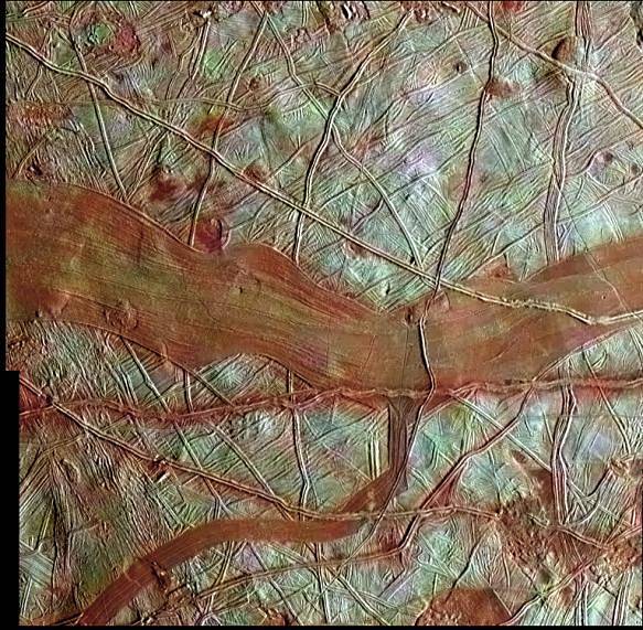
Tag: CFD

  • Flow in the Heart

    Flow in the Heart

    Few flows are more integral to our well-being than blood flow through the heart. Over the course of our lives, our hearts develop from a few cells pushing viscous blood through tiny arteries to the muscular center of a vast circulatory network, capable of powering us through incredible physical feats. What’s most astonishing about all this is that the heart goes through all these changes and adaptations without ever pausing. 

    Peering into the heart to see it in action is difficult, but researchers today are combining imaging techniques like CT and MRI with computational fluid dynamics to build patient-specific heart models. Not only does this help us understand hearts in general; it’s paving the way toward predicting how a specific treatment may affect a patient. Imagine, for example, being able to simulate and compare different models of an artificial heart valve to see which will work best for a particular patient. We’re not to the point of doing so yet, but it’s a very real possibility in the future. 

    To see some examples of predicted and measured heart flows, check out this video by J. Lantz. In the meantime, happy Valentine’s Day! (Image credits: Linköping University Cardiovascular Magnetic Resonance Group, video source; via Another Fine Mesh)

  • Inside a Heart

    Inside a Heart

    You may not give it much thought, but there is important fluid dynamics happening inside you every moment of every day, especially inside your heart. Of the four chambers of the heart, the left ventricle has the thickest walls, reflecting its important task: pumping oxygenated blood throughout the body. In a healthy heart (top of poster; click here for the full-size version), a vortex ring and trailing jet fill the ventricle when the mitral valve opens. Then the ventricle contracts and pumps blood out the aortic valve and into the rest of the body.

    But for individuals with a leaking aortic valve (bottom of poster), things look different. Blood leaks back through the aortic valve at the same time that the mitral valve opens to allow freshly oxygenated blood back in. The two inflows disrupt mixing in the chamber, and, instead of pumping fully-oxygenated blood into the body, the left ventricle has to struggle to pump a less-oxygenated mixture into the body. (Image credit: G. Di Labbio et al.)

    ETA: (Research paper: G. Di Labbio et al., arXiv)

  • What Makes Turbulence So Hard

    What Makes Turbulence So Hard

    Turbulence – that pestersome, unpredictable, and chaotic state of flow – has been a thorn in the sides of mathematicians, physicists, and engineers for centuries. It is certainly one of – if not the – oldest unsolved problem in physics. Over at Ars Technica, Lee Phillips has a nice overview of the situation, including what makes the problem so difficult:

    The Navier-Stokes equation is difficult to solve because it is nonlinear. This word is thrown around quite a bit, but here it means something specific. You can build up a complicated solution to a linear equation by adding up many simple solutions. An example you may be aware of is sound: the equation for sound waves is linear, so you can build up a complex sound by adding together many simple sounds of different frequencies (“harmonics”). Elementary quantum mechanics is also linear; the Schrödinger equation allows you to add together solutions to find a new solution.

    But fluid dynamics doesn’t work this way: the nonlinearity of the Navier-Stokes equation means that you can’t build solutions by adding together simpler solutions. This is part of the reason that Heisenberg’s mathematical genius, which served him so well in helping to invent quantum mechanics, was put to such a severe test when it came to turbulence. 

    Phillips goes on to describe some of the many methods researchers use to unravel the mysteries of turbulence computationally, experimentally, and theoretically. This is a great introduction for those curious to get a sense of how turbulence, stability theory, and computational fluid dynamics all fit together. (Image credits: L. Da Vinci; NASA; see also: Ars Technica; submitted by Kam Yung-Soh)

  • Featured Video Play Icon

    Swimming, Cycling, and Sailing

    Summer brings with it lots of great sports, and whether you love riding a bike, sailing a boat, or just hanging out at the pool, our latest FYFD/JFM video has something for you. Want even more sports physics? Check out the Olympic series we did for the London and Rio games. And if you’re looking for more of the latest fluids research, don’t miss the rest of our video series. (Video and image credit: N. Sharp and T. Crawford)

  • Breaking With a Wave

    Breaking With a Wave

    For rocket combustion and other applications, like watering your lawn with a hose, a stream of fluid may need to be broken up into droplets. While simply spraying a liquid jet will make it break up, waving that jet back and forth will break it up faster. A recent study simulated this problem numerically to determine the exact mechanisms driving that break-up. The researchers found two major culprits.

    The first is a Kelvin-Helmholtz, or shear-based, instability. When a jet leaves the nozzle, there’s friction between it and the comparatively still air surrounding it. This creates tiny ripples in the surface that eventually grow into the distortions we can see, and it’s found in all jets, regardless of their side-to-side motion.

    The second culprit, which is only found in the oscillating jet, is a Rayleigh-Taylor instability. By moving the jet side-to-side, you’re driving the dense liquid into less dense air, which creates a different set of disturbances that also help break up the jet. The final result: swinging the jet side-to-side breaks it into smaller droplets faster. (Image and research credit: S. Schmidt et al.)

  • Forming Europa’s Bands

    Forming Europa’s Bands

    Jupiter’s icy moons, Europa and Ganymede, are home to subsurface oceans. These moons also experience strong tidal forces from their parent planet and sibling moons that squeeze and deform them over time. A new study focuses on the bands, seen in red in the top image of Europa, that form as a result of these deformations. By simulating (bottom image) both the convective currents within the Europan ocean and the deformation of the ice over time, scientists are able to study how these geological surface features may have formed. Over the course of about a million years, material from the interior ocean works its way up into the center of a band. Because this process takes so long, the researchers point out that any attempt to collect material from the bands will yield “fossil” ocean material – essentially a glimpse of Europa’s ocean as it existed a million years ago rather than how it exists today! (Image credit: NASA; image and research credit: S. Howell and R. Pappalardo, source; submitted by Kam-Yung Soh)

  • Prehistoric CFD

    Prehistoric CFD

    Computational fluid dynamics (CFD) has been a valuable tool in engineering for decades, but its use is spreading to other fields as well. The image to the left shows a reconstruction of Parvancorina, a shield-shaped marine creature that lived some 550 million years ago. Fossil evidence alone cannot tell paleontologists whether this extinct creature could move through the water, and there are no living relatives that resemble the creature that scientists could study as an analogue. Instead, researchers turned to CFD to simulate flow over and around Parvancorina. They found that Parvancorina’s shape caused fast flow over the outer portions of its body and the slowest flow near its mouth. The results suggest that, not only was the creature mobile in the water, but that it was able to adjust its orientation to drive flow to different areas of its body. Paleontologists have only been using CFD for a decade or so, but already it’s giving us valuable insight into the creatures that roamed our planet hundreds of millions of years ago. (Image credit: M. De Stefano/Muse, I. Rahman; via Physics Today)

  • Adaptive Meshing

    Adaptive Meshing

    The use of numerical simulations in fluid dynamics has exploded over the past half century with new computational techniques being developed constantly. Most methods involve solving the equations of motion (or an approximation thereof) on a grid of points known as a mesh. To accurately capture the physics, meshes must often be quite closely packed in areas where detail is needed, but they can be more widely spaced in areas where the flow is not changing quickly. An increasingly common technique is adaptive meshing in which the mesh of grid points shifts between time steps; this places more grid points where the flow requires them and removes them from less important areas in order to reduce computational time.

    An example of adaptive meshing is shown above. On the left particles are falling into salt water. The colors show the concentration of particles. The right side shows the solid particles and the fluid mesh around them. Notice how the grid shifts as the particles fall. (Image credit: C. Jacobs et al., source)

  • Featured Video Play Icon

    Inside Earth’s Core

    Without our magnetic field, life as we know it could not exist on Earth. Instead, our atmosphere would be stripped away and the surface would be bombarded by charged particles in the solar wind. Relatively little is known about the dynamo process that governs our magnetic field, though it’s thought to be the result of liquid iron moving in the Earth’s outer core. The video above shows a slice of a recent 3D simulation of this liquid iron segment of our core. The colors show variations in the temperature, revealing vigorous convection in the core. This motion, combined with the spinning of the Earth, is the likely source of our magnetic field. Researchers hope that simulations like these can help us understand features we observe in our magnetic field – like local variations in field strength and the pole reversals in our geological record. (Video credit: N. Schaeffer et al.; CNRS via Gizmodo)

  • Break-Up of the Chelyabinsk Meteor

    Break-Up of the Chelyabinsk Meteor

    In 2013, a meteor about 20-meters in diameter broke up over Chelyabinsk, Russia in a dramatic display that damaged buildings within 100 km and injured more than 1200 people. To better understand the threat presented by such objects, NASA has been conducting 3D, hypersonic simulations like the one shown here. The meteor material is shown in gray and black. Brighter colors like red and yellow indicate the hot, high-pressure shock wave caused when the meteor slams into the atmosphere. Aerodynamic effects quickly erode the meteor, ripping it into pieces that disperse energy explosively in the atmosphere. While you might think the meteor breaking up is good for us, it’s actually the blast waves from its break-up that cause the most damage.  (Image and video credit: NASA, source; via Gizmodo)